Introduction
This is the second post in a two part series regarding the implementation of graph-tool in an environment where it can interact with a peartree network graph. To learn more about how the installation was performed, please see this blog post for the installation notes.
The purpose of this post is to describe how to take a peartree network and convert it to a graph-tool object. This means transferring over all nodes and edges and all attributes related to each. If you google how to do this (with a query like “convert networkx graph to graph-tool”), the best result will be this terrific blog post from a little over 2 years ago (middle of 2016).
While this post is a great (the author back then also acknowledged what a PIA it was to set up, stating: “It’s a bear to get setup, but once you do things get pretty nice. Moving my network viz over to it now!” - link to Tweet), it’s in Python 2 and some aspects of graph-tool have changed slightly.
Advantage of peartree on graph-tool
graph-tool is much faster than NetworkX at evaluation. NetworkX implements graph-algorithms in pure Python and thus trades perforamnce for ease of use. On more complex networks, performance hits can make iterative development difficult or impossible. graph-tool frees up operations to take advantage of parallelization, as well as the traditional advantages of lower level code to perform computation-intensive operations more quickly and efficiently than pure Python approaches.
Let’s look at an example. A common measure of a graph that I perform is the evaluation of betweenness centrality. Here are the results of performing this operation on an identical graph, once in NetworkX and once in graph-tool:
Stats for network graph being evaluated:
- Nodes: 4,969
- Edges: 5,554
Performance on NetworkX: 2min 34s Performance on graph-tool: 756 ms
Relative performance gain for this graph: 203,703.7% faster.
Clearly, graph-tool is the winner in this comparison. For more details on graph-tool’s performance, be sure to check out the project’s own documentation on this, here.
Acknowledging original authorship
In this post, I seek to update the original post’s method and make comments on those changes. In addition, I will be using a peartree network instead of a simple, arbitrary NetworkX graph. That said, thanks to the author, Benjamin Bengfort for his work, which I am merely regurgitating with slight modification here.
Converting from NetworkX to graph-tool
Again, the logic will largely be similar to what was set out in the source blog post. I will just be making note of some modifications made to get this to play with Python 3.
First, the get_prop_type method has been updated. This method is used to process the outputs of the graph elements that are returned from graph-tool’s Python API. The returned objects, particularly string-like values, are returned encoded as bytes so it is necessary to produce a helper function to handle these types before continuing with process logic. Specifically, the changes are meant to ensure that the key is not converted to ASCII but instead decoded to a Python 3 string type. The same goes for the value parameter.
The method now looks like this:
def get_prop_type(value, key=None):
    """
    Performs typing and value conversion for the graph_tool PropertyMap class.
    If a key is provided, it also ensures the key is in a format that can be
    used with the PropertyMap. Returns a tuple, (type name, value, key)
    """
    # Ensure that key is returned as a str type
    if isinstance(key, bytes):
        key = key.decode()

    # Deal with the value
    if isinstance(value, bool):
        tname = 'bool'

    elif isinstance(value, int):
        tname = 'float'
        value = float(value)

    elif isinstance(value, float):
        tname = 'float'

    elif isinstance(value, bytes):
        tname = 'string'
        value = value.decode()

    elif isinstance(value, dict):
        tname = 'object'

    else:
        tname = 'string'
        value = str(value)

    return tname, value, key
Now that we have a method to handle processing output variable types from interfacing with the items from graph-tool, we can largely preserve the logic developed by Benjamin Bengfort from his previous blog post.
I’ve copied the method, here, for reference. Minor updates (primarily related to updates to the NetworkX node and edge iteration API) were made to make the script Python 3 compatible.
def nx2gt(nxG):
    """
    Converts a networkx graph to a graph-tool graph.
    """
    # Phase 0: Create a directed or undirected graph-tool Graph
    gtG = gt.Graph(directed=nxG.is_directed())

    # Add the Graph properties as "internal properties"
    for key, value in nxG.graph.items():
        # Convert the value and key into a type for graph-tool
        tname, value, key = get_prop_type(value, key)

        prop = gtG.new_graph_property(tname) # Create the PropertyMap
        gtG.graph_properties[key] = prop     # Set the PropertyMap
        gtG.graph_properties[key] = value    # Set the actual value

    # Phase 1: Add the vertex and edge property maps
    # Go through all nodes and edges and add seen properties
    # Add the node properties first
    nprops = set() # cache keys to only add properties once
    for node, data in nxG.nodes(data=True):

        # Go through all the properties if not seen and add them.
        for key, val in data.items():
            if key in nprops: continue # Skip properties already added

            # Convert the value and key into a type for graph-tool
            tname, _, key  = get_prop_type(val, key)

            prop = gtG.new_vertex_property(tname) # Create the PropertyMap
            gtG.vertex_properties[key] = prop     # Set the PropertyMap

            # Add the key to the already seen properties
            nprops.add(key)

    # Also add the node id: in NetworkX a node can be any hashable type, but
    # in graph-tool node are defined as indices. So we capture any strings
    # in a special PropertyMap called 'id' -- modify as needed!
    gtG.vertex_properties['id'] = gtG.new_vertex_property('string')

    # Add the edge properties second
    eprops = set() # cache keys to only add properties once
    for src, dst, data in nxG.edges(data=True):

        # Go through all the edge properties if not seen and add them.
        for key, val in data.items():
            if key in eprops: continue # Skip properties already added

            # Convert the value and key into a type for graph-tool
            tname, _, key = get_prop_type(val, key)

            prop = gtG.new_edge_property(tname) # Create the PropertyMap
            gtG.edge_properties[key] = prop     # Set the PropertyMap

            # Add the key to the already seen properties
            eprops.add(key)

    # Phase 2: Actually add all the nodes and vertices with their properties
    # Add the nodes
    vertices = {} # vertex mapping for tracking edges later
    for node, data in nxG.nodes(data=True):

        # Create the vertex and annotate for our edges later
        v = gtG.add_vertex(n=1)
        vertices[node] = v

        # Set the vertex properties, not forgetting the id property
        data['id'] = str(node)
        for key, value in data.items():
            tname, value, key = get_prop_type(value, key)
            gtG.vp[key][v] = value # vp is short for vertex_properties

    # Add the edges
    for src, dst, data in nxG.edges(data=True):

        # Look up the vertex structs from our vertices mapping and add edge.
        e = gtG.add_edge(vertices[src], vertices[dst])

        # Add the edge properties
        for key, value in data.items():
            gtG.ep[key][e] = value # ep is short for edge_properties

    # Done, finally!
    return gtG
Convert a peartree network graph
Now that we’ve ported the script over to be compatible with both newer versions of NetworkX and Python 3, we can attempt to port a peartree graph output to graph-tool and play with it.
First, let’s parse a GTFS feed with peartree. I’ve probably written this step a million times now, but getting a peak hour network graph from peartree is pretty straightforward. Let’s work with AC Transit’s GTFS:
import peartree as pt

path = 'gtfs/ac_transit.zip'
feed = pt.get_representative_feed(path)
start = 7*60*60  # 7:00 AM
end = 8*60*60  # 10:00 AM
G = pt.load_feed_as_graph(feed, start, end, use_multiprocessing=False)
At this point, it is straightforward to plot the system and take a look at what we have:
pt.plot.generate_plot(G)The above plot script should return this image:
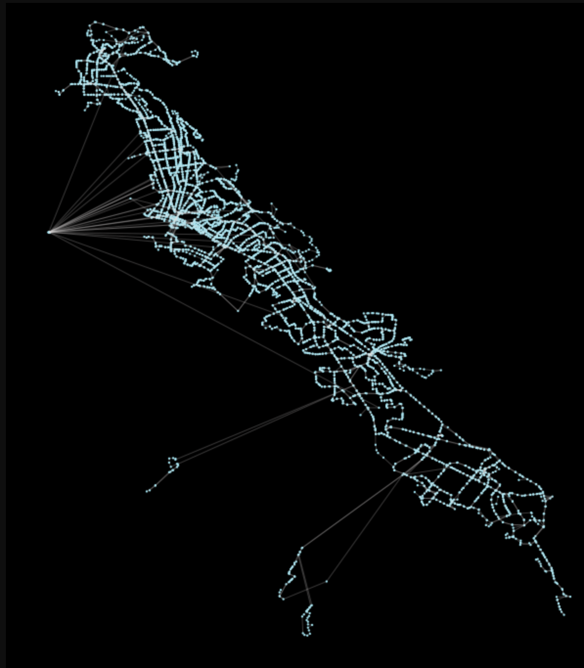
This is the AC Transit system, covering the East Bay of the San Francisco metro area, represented as a network graph.
At this point, we can take that graph and convert it to a graph-tool graph with our new conversion script.
nxG = G.copy()
gtG2 = nx2gt(nxG)
graph_draw(gtG2)
Terrific. This output should produce a graph plot that looks something like the below:
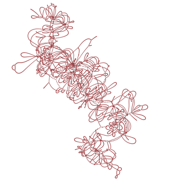
This layout is somewhat arbitrary. Without any specified positions, the network graph will attempt to determine an optimum layout using an algorithm, Scalable Force Directed Placement (SFDP), which is available as part of the graphviz software (installed in the previous post).
Alternative rendering
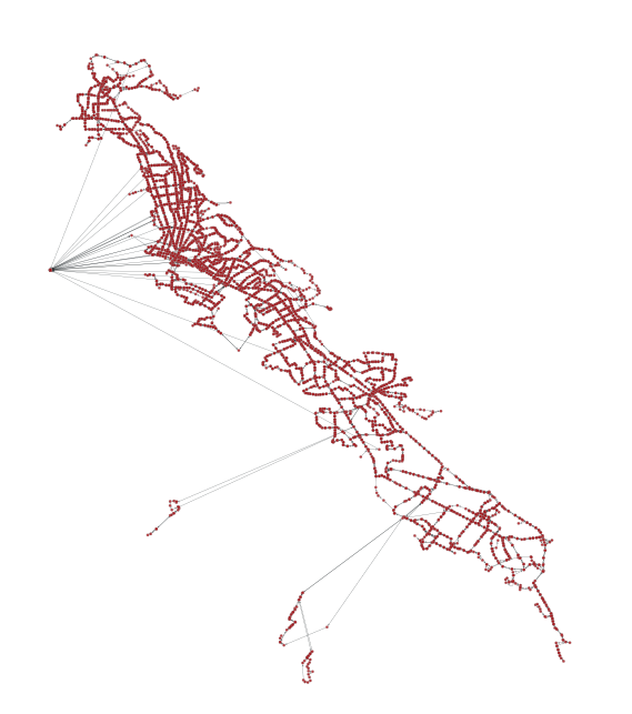
If we’d like to plot the locations based off of the x/y values from the original networks stop positions, we can do so by creating a new PropertyMap and adding it to the vertices:
tname = 'vector<float>'
key = 'loc'

prop = gtG2.new_vertex_property(tname)
gtG2.vertex_properties[key] = prop
In this method, we assign the type for this new property map to be a vector, holding two values (x and y) under the key loc.
Now, we can iterate through those values and add them to the network graph, like so:
vs = [int(v) for v in gtG2.vertices()]
locs = zip([x for x in gtG2.vp['x']], [y for y in gtG2.vp['y']])

for v, loc in zip(vs, locs):
    gtG2.vp[key][v] = loc
The output should look similar to our initial plot, from peartree’s first load of the network from AC Transit’s GTFS:
Betweenness centrality
Similarly, we can plot betweenness centrality (or any of a host of other graph algorithms) through graph-tool’s API. With betweenness, we first import the method to calculate this measures impact on both edges and vertices:
from graph_tool.centrality import betweenness
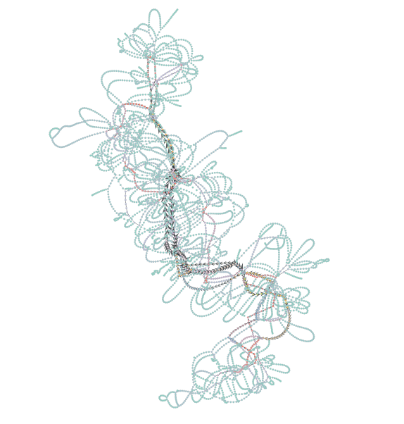
bv, be = betweenness(gtG)Having acquired these new vertices and edge values, we can recalculate the SFDP layout with these modified edge values in consideration.
from graph_tool.draw import sfdp_layout
pos = sfdp_layout(gtG, eweight=be)
With those new positions, we can replete the graph, and also use the vertex and edge calculations to inform line width, to help add some further visual clarity:
graph_draw(gtG, pos=pos, vertex_fill_color=bv, edge_pen_width=be)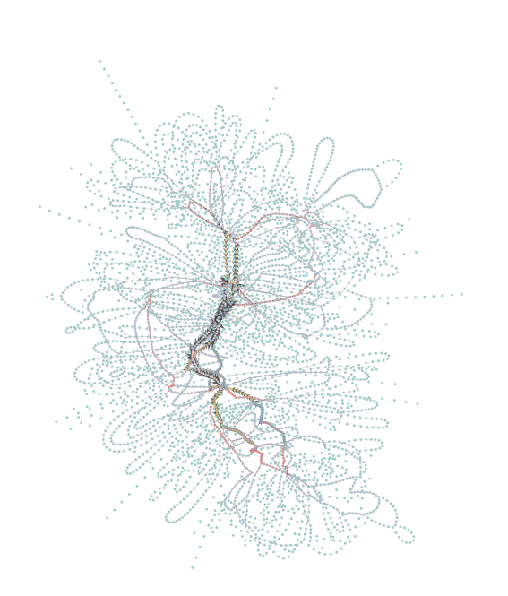
This produces quite a nice result, where the core of the AC Transit network (and the hinge around downtown Oakland) are particularly visible.
Hope this post helps with other folks looking to obtain higher performance tooling with graph-tool, particularly those working with peartree. Moving forward, I’d like to explore implementation of accessibility algorithms via graph-tool to enable an “all-in-one” approach to network accessibility measures from just peartree on top of graph-tool.