Introduction

In this post I demonstrate how one can leverage mesh grids in numpy and series of centroid-related float value data to perform vectorized operations that result in index pairs. These index pairs can then group the original geometry collection into cell clusters for more performant, matrix-based calculations that circumvent full spatial analytics bottlenecks.

Background

It is common in spatial analysis methodology to want to perform buffering and clustering operations. For example, I may have a dataset of all lots in a given city and I want to know, for each parcel, what the average number of households there are, per parcel, in the surrounding quarter mile. At times, I may also want to know the amount of some attribute within a variable distance, where the determinant of buffer radius is an attribute associated with each parcel.

# pseudocode for how a simple iteration might occur
for geometry in all_geometries:
    all_distances = geometry.distance(all_geometries)
    subset = ref_frame[all_distances < one_mile]
    do_something(subset[target_attribute].mean())

In such instances, the standard operation is to iterate through each geometry in the list of all geometries (e.g. all parcels) and identify all that lie within range N of that target geometry. As the number of geometries increases, this operation can become very expensive. One way to assist in improving performance is to use an Rtree spatial index. This allows the entire set of geometries to be indexed, which makes identifying likely candidates for intersection with a buffered geometry to be made more quickly, based off the bounds of each of all other geometries.

Another improvement is to use centroids. Using the centroids, one can calculate distances more cheaply, considering only a single vertices for each point:

# pseudocode for how a simple iteration might occur
# that now uses centroids
all_centroids = all_geometries.centroids

for centroid in all_centroids:
    all_distances = all_centroids.distance(centroid)
    subset = ref_frame[all_distances < one_mile]
    do_something(subset[target_attribute].mean())

Given that these values are just two float values, the data can be vectorized as two numpy arrays (if you are using Python) and factored that way. This leverages the advantage of vectorized arrays in Python, which avoids the costly for loops that are present inside other Python tools (e.g. Shapely).

Ultimately, regardless of the methodology, this inherently involves calculation of a distance matrix. This has intrinsic performance costs (it is exponentially increasing in computation costs as the array length of geometries increases). I’ve dived into implementations of tackling this method using Python, Cython, and Julia in another blog post if you’d like to dive into this further.

Example dataset

We will be using the parcel dataset that San Francisco makes available as an example. You can download it from there open data portal, here.

The requirements we will need to perform all the work described below is pretty bare bones:

import geopandas as gpd
import matplotlib.pyplot as plt
import numpy as np

Go ahead and read the dataset in with GeoPandas as then recast to a meter based projection for the sake of ease of geometry manipulation in later steps:

gdf = gpd.read_file('sf_parcels')

# Apparently there are a few bad geometries in the dataset
mask = [g is not None for g in gdf.geometry]
gdf = gdf[mask]

gdf.crs = {'init': 'epsg:4326'}
gdf.geometry = gdf.geometry.buffer(0)
gdf = gdf.to_crs(epsg=3857)

Now, for the slowest part of this whole operation. Extract the centroids from the dataframe. This takes 11 seconds on my machine (2015 MacBook Pro, 13”, in a Docker container with access to two CPUs, 12 GB of RAM).

# Get xs and ys for all centroids
centroids = gdf.centroid
cxs = centroids.map(lambda c: c.x).values
cys = centroids.map(lambda c: c.y).values

Now that we have the x and y values, we are “free” from being tether to geospatial data and can move on to purely vectorized operations. The rest of this post is going to be Python specific (it is about numpy, after all).

Cell clustering algorithm

First we need to extract the min and max values from the x and y series:

xmin = cxs.min()
ymin = cys.min()
xmax = cxs.max()
ymax = cys.max()

Next, we should shift the whole series of x and y values so that the “bottom left” point is at (0,0). This will allow us to cleanly convert each geometry centroid to its relative index for its corresponding cell (assuming that the cells are arranged in such a way where cell index (0,Y) sits atop the location of the “leftmost” geometries (the geometries that has the smallest x values).

These adjusted values are then divided by the grid width and rounded down to the nearest floor integer value. This gets us the index of the cell that this centroid can be paired with.

cxs_adj = np.floor((cxs - xmin) / grid_width).astype(int)
cys_adj = np.floor((cys - ymin) / grid_width).astype(int)

Now that we have adjusted x and y values such that all are relative distances to a base (0,0) value, we just need to determine the shape of the overall project site that the adjusted centroid values are the indices for. This shape will be used to generate a 2 dimensional matrix of zero values representing the grid cells for the region.

xmin_adj = xmin - xmin
ymin_adj = ymin - ymin
xmax_adj = xmax - xmin
ymax_adj = ymax - ymin

mesh_x_points = np.mgrid[xmin_adj:xmax_adj:grid_width]
mesh_y_points = np.mgrid[ymin_adj:ymax_adj:grid_width]

mesh_shape = (mesh_x_points.shape[0], mesh_y_points.shape[0])
totals = np.zeros(mesh_shape)

With a grid width of 150 meters, we only create 12,320 cells so iteration through this becomes fairly trivial.

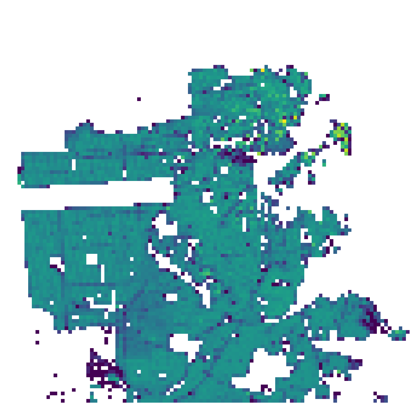
In fact, in this situation, we can just for loop through the dataset and get sums based off of whatever target attribute we are interested in. For example, the parcels dataset has a land use designation (zoning I think) under the column districtna. We can include this as we iterate through the cells to calculate density of, say, residential related zoning parcels in the city:

for all_vars in zip(cxs_adj, cys_adj, gdf.districtna):
    i = all_vars[:2]
    dna = all_vars[2]
    if dna and 'RESIDENTIAL' in dna:
        totals[i[0], i[1]] += 1

The resulting output shows a reasonable resolution, and neighborhoods are clear from the plot:

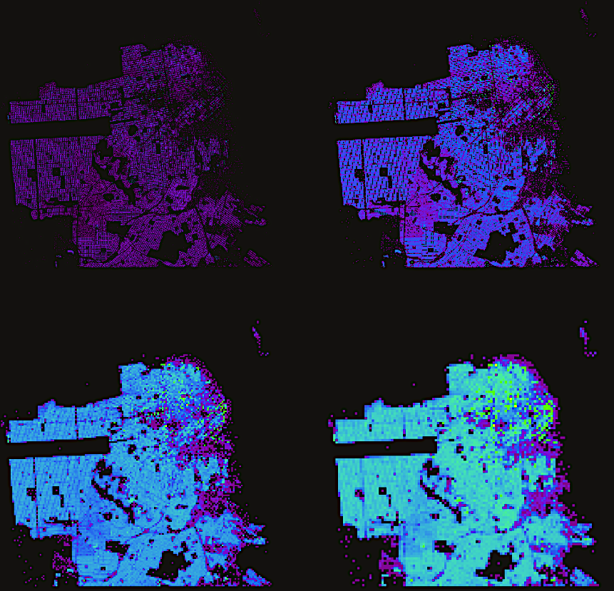
Varying grid width

While the above result was great, what is handy about this method is that it is really fast! The entire operation runs in about 1/5th of a second on my machine, which makes running and comparing results at various grid widths a breeze. Below, I test out 25, 50, 100, and 150 meter grid widths:

xmin = cxs.min()
ymin = cys.min()
xmax = cxs.max()
ymax = cys.max()

xmin_adj = xmin - xmin
ymin_adj = ymin - ymin
xmax_adj = xmax - xmin
ymax_adj = ymax - ymin

totals = {}
for grid_width in grid_widths:
    cxs_adj = np.floor((cxs - xmin) / grid_width).astype(int)
    cys_adj = np.floor((cys - ymin) / grid_width).astype(int)

    mesh_x_points = np.mgrid[xmin_adj:xmax_adj:grid_width]
    mesh_y_points = np.mgrid[ymin_adj:ymax_adj:grid_width]

    mesh_shape = (mesh_x_points.shape[0], mesh_y_points.shape[0])

    totals[grid_width] = np.zeros(mesh_shape)

    for i in zip(cxs_adj, cys_adj):
        totals[grid_width][i] += 1

Iterating through this 4 times took me about 0.6 seconds. As you can see, reaching fairly high resolutions is fairly trivial and allows for modeling reasonable large areas with a fairly minimal memory overhead. Ultimately, it becomes more a matter of determining the best grid width (perhaps more an art than a science) based off heuristics associated with the typical profile of the geometries you are dealing with (e.g. parcels, vs. Census blocks, vs. TAZs, etc.).

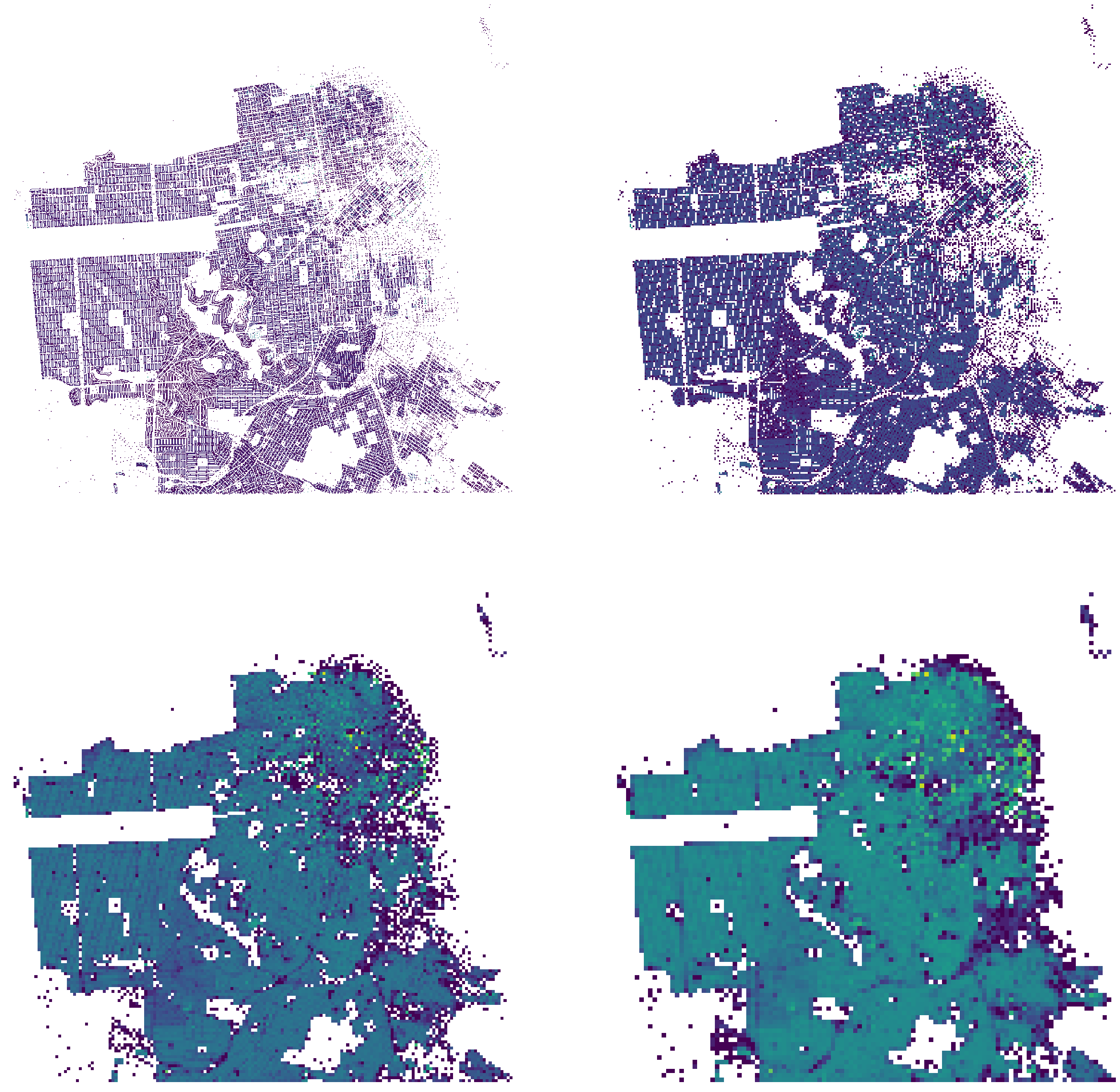
Script to generate the plots looks like this:

def convert(t_vals):
    return np.rot90(np.reshape(np.log(t_vals), t_vals.shape))

fig, axarr = plt.subplots(2, 2, figsize=(48,48))

arr_is = [[0, 0], [0, 1], [1, 0], [1, 1]]
for i, gw in zip(arr_is, grid_widths):
    axarr[i[0], i[1]].imshow(convert(totals[gw]), cmap=plt.cm.viridis)
    axarr[i[0], i[1]].axis('off')