Performing geospatial operations in Python can be a slow and tedious process. Tools for handling spatial data in Python (specifically GeoPandas, which supplies Pandas Dataframes with spatial capabilities on geometry columns containing Shapely objects) that are highly effective during the exploratory phase can fall short when performing on larger datasets. For example, a common use case I have run into is running a series of geometric operations in which, given a GeoPandas GeoDataFrame, I need to perform some arithmetic operation on a subset of the total data frame comprised of all rows within or intersecting a varying range (buffer) of a given row’s geometry. This need to be performed on each row in the data frame, for each subsequent analysis.
Performance hinderances with larger geo-datasets
This operation can quickly raise problems. For example, given a data frame of ~50,000 rows, an operation in which each geometry can be buffered by varying lengths can dozens of minutes to complete. Factor that by a nested series of operations (often called a DAG, or directed acyclic graph) each of which requires a full pass through of all geometries against all rows, and an analytics process can balloon to the tens of hours.
Below, an example of a typical row-wise operation involving all geometries on the GeoDataFrame in each row’s applied method:
def rowwise_operation(row):
    # determine some coefficient based off row attributes
    a = row.attribute_a
    b = row.attribute_b
    special_coeff = factor_multiple_row_attributes(a, b)

    # use that result to determine a variable bounding distance
    buffered_geom = row.geometry.buffer(special_coeff)

    # get the subset of the geodataframe that intersects with that buffer
    does_intersect = example_geodataframe.geometry.intersects(buffered_geom)
    subset_example = example_geodataframe[does_intersect]

    # derive some value from that result
    foo = subset_example.attribute_foo.sum()
    bar = subset_example.attribute_bar.sum()

    return (row.id, foo, bar)

example_geodataframe.apply(rowwise_operation, axis=1)
Optimization through utilization of an R-tree spatial index
There is relief for optimizing analyses on large geometries and GeoPandas supports this. Most significantly, an R-tree spatial index can be generated that essentially enables most geometries to be tossed before a full intersection of distance calculation is performed by indexing all geometries into a series of reference bounding boxes. You can read more about spatial indexing here.
 Above, a visualization of a what an R-tree might look like spatially, where proximity is used to identify clusters of geometries by proximity/zone. You can read more on this OSM Open Layers blog post.
Below, an example implementing the spatial index to assist in speeding up a typical geospatial operation:
si = example_geodataframe.sindex
def rowwise_operation(row):
    # determine some coefficient based off row attributes
    a = row.attribute_a
    b = row.attribute_b
    special_coeff = factor_multiple_row_attributes(a, b)

    # use that result to determine a variable bounding distance
    buffered_geom = row.geometry.buffer(special_coeff)

    # get the subset of the geodataframe that intersects with that buffer
    # utilizing the spatial index to toss all absolute outliers out first
    possible_matches_index = list(si.intersection(buffered_geom.bounds))
    possible_matches = example_geodataframe.iloc[possible_matches_index]

    # perform prior steps and continue as before
    does_intersect = possible_matches.geometry.intersects(buffered_geom)
    subset_example = possible_matches[does_intersect]

    # derive some value from that result
    foo = subset_example.attribute_foo.sum()
    bar = subset_example.attribute_bar.sum()

    return (row.id, foo, bar)

example_geodataframe.apply(rowwise_operation, axis=1)
Unfortunately, the introduction of spatial indexing can only improve the performance of these operations so much. One of the major blockers to performance in Pandas (and, of course, Python generally) is the presence of for loops. Iterating through all rows in a GeoDataFrame is expensive, regardless of the presence of a spatial index. Ultimately, performance gains must be gained by parallelizing this process.
Opportunities for parallelization
Because each row’s output can be calculated independently, this falls squarely within the definition of an embarrassingly parallel workload. Essentially, if I had n rows, I could run n parallel processes and calculate the distance from one geometry to another (or all others) at the same time, thus drastically reducing the completion time for the operation at the cost of some additional resources for the overhead required to reduce those parallelized processes all back into a single result.
Parallelization also offers an additional opportunity. Calculating the distance between a given geometry and all other geometries is expensive in Python. Previously, utilization of the R-tree was critical because it meant that each row-wise operation (which involved calculating all possible intersecting geometries within the entire data frame) was expensive (effectively a nested for loop). Parallelization, on the other hand, offers an opportunity to calculate the distance between each geometry and all other possible geometries. This is advantageous as it allows us to produce a float value for each unique id pairing (e.g. geometry ID_194 and geometry ID_3047).
Utilization of a distance matrix
Once distances between all geometries to all geometries has been calculated, the results can be stored in a variety of compressed methods. A 50,000 row GeoDataFrame converted to all unique key combinations is over 2.5 billion rows long. This is not possible to be stored as a dataframe. That said, a dictionary of 50,000 keys, each holding a Numpy array of length 50,000 containing an ordered list of the lengths to all other geometries in the network is feasible. Other options exist as well, including sorting the data into categorized csvs and only reading in the segment of the resulting distances that is relevant to a given geometry’s ID. This blog post will not cover the different storage solutions, suffice to say there are many paths forward and one may be more or less appropriate given your context.
The advantage of a distance matrix is that, once the many-to-many distances have been calculated, we are free to take advantage of opportunities to vectorize what were previously not-vectorizable operations, namely all the geometric comparisons. Let’s go back to the example function shown earlier, before we introduced the spatial index. Instead of utilizing a spatial index, we could simply ask for the Numpy array of all distances from one geometry to all others in the network and then ask for only the ids of the other geometries that are within a certain distance of the first geometry. The resulting booleans array from the distance array would make returning these results very quick, removing the need for geospatial comparisons to be made during the operation of the applied function entirely.
Below, an example of how this might look were we to modify the above example function:
def rowwise_operation(row):
    # determine some coefficient based off row attributes
    a = row.attribute_a
    b = row.attribute_b
    special_coeff = factor_multiple_row_attributes(a, b)

    # use that result to determine a variable bounding distance
    buffered_geom = row.geometry.buffer(special_coeff)

    # get the subset of the geodataframe that intersects with that buffer
    # utilizing the precalculated distance matrix, which is a Numpy array, and
    # thus far more performant than the previous geometric comparison method
    within_ids = PreGeneratedDistMatrix.get_geoms_within_dist_of(row.id, special_coeff)
    possible_matches = example_geodataframe.iloc[possible_matches_index]

    # perform prior steps and continue as before
    subset_example = possible_matches[possible_matches.ids.isin(within_ids)]

    # derive some value from that result
    foo = subset_example.attribute_foo.sum()
    bar = subset_example.attribute_bar.sum()

    return (row.id, foo, bar)

example_geodataframe.apply(rowwise_operation, axis=1)
How to parallelize geospatial processes in Python
A relatively recent library, Dask, has made parallelization in Python quite simple. In the below example, I will demonstrate how one might set up Dask to parallelize the generation of a distance dictionary. The data being used in the following examples can be downloaded from my Dropbox, here. It’s a generic csv with three self-explanatory columns: id, value, geometry. The geometry column is stored as a WKT (well-known text file), which can be converted to a Shapely geometry object via the library’s wkt.loads load string method.
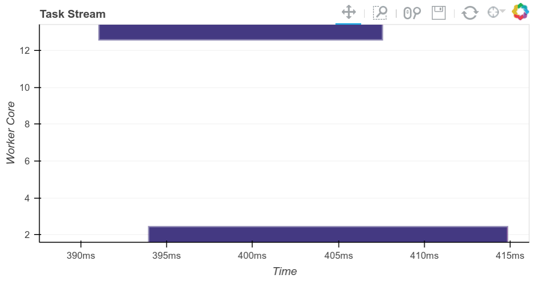 Matthew Rocklin, the primary creator of Dask, has written about it extensively and created a number of really helpful visualizations, such as the above, to demonstrate the Scheduler’s orchestration of tasks to map jobs out to workers and reduce results back when requested. You can read more on his blog.
Here’s a quick example of how one might normally generate this distance dictionary:
import geopandas as gpd
import numpy as np
import pandas as pd
from shapely.wkt import loads
from timeit import timeit

# take a subset of the dataframe (df) per increment
df = pd.read_csv('./example_geometries.csv').head(1000)

def convert_to_gdf(df):
    # given a pandas dataframe, return a geopandas geodataframe
    geometries = gpd.GeoSeries(df['geometry'].map(lambda x: loads(x)))

    # take a subset of the pandas df and convert to a gdf via geopandas
    gdf = gpd.GeoDataFrame(data=df[['id', 'value']],
                           crs={'init': 'epsg:32154'},
                           geometry=geometries)

    return gdf

# convert the pandas df to a geo df
gdf = convert_to_gdf(df)

def generate_distance_matrix():
    print('Beginning to calculate distance matrix...')
    distances_dict = {}
    for row in gdf.itertuples():
        row_id = row[1]
        row_geom = row[3]
        all_dists = gdf.geometry.distance(row_geom)
        distances_dict[row_id] = np.array(all_dists)
    print('Completed calculating distance matrix.')
    return distances_dict

# execute the operation
t = timeit(generate_distance_matrix, number=1)
print('Runtime: {}s'.format(t))
As you can see, the above operation is deeply flawed. Attempting to create a distance dictionary with the above method would be an extremely time consuming endeavor. Faced with this option alone, the spatial index path is naturally preferable.
Now, with Dask, we will need to make sure two libraries are installed (Dask, Distributed). The latter, Dask.distributed, is a centrally managed, distributed, dynamic task scheduler. Setting it up can be as hands-off or as hands-on as you want (part of Dask’s strong appeal).
I’ll save a deeper dive into Dask for another post, but suffice to say that Dask Distributed makes it easy for one to spin up external resources, sync up to them with Dask Scheduler, and then run parallelized jobs across multiple workers.
Briefly, once you have Dask installed, open a terminal window and wherever it is installed and run dask-scheduler in the command line prompt. It will log information on how to access it immediately after. The log should look something like Scheduler at: tcp://{some_address}:8786 where some_address is the location of the service that is running the scheduler.
Locally, in your Python script, you should be able to access it now via Dask Distributed’s Client object as in the below example:
from dask.distributed import Client
client = Client('tcp://{some_address}:8786')
Once you’ve secured a connection, make sure to spin up as many workers as you need. Each worker can be directed to the scheduled in the same way as the Class object from Distributed:
dask-worker {some_address}:8786Once a connection has been secured feel free to load in your data frame as before, in Pandas. As with the before example, we will subset the data frame for the purposes of working through the example. The subsetting portion can be removed when analysis on the full dataset is desired.
subset_length = 1000
df = init_df.head(subset_length)
df = df.assign(temp_key=1).reset_index(drop=True)
In addition to loading in the dataset, you may have noticed we also assigned a new column temp_key. This will be used in just a moment. Before we do, we want to create a Dask version of the Pandas data frame as well.
ddf = dd.from_pandas(df, npartitions=10) Note that we have no converted this to a GeoDataFrame. As a result, the column holding the WKT geometries is simply plain text as far as Dask and Pandas are concerned right now. This is because Dask does not support GeoPandas and because conversion of the tall all-to-all data frame to a GeoDataFrame would be both unnecessary and very expensive.
The partition count is up to you. If you have three workers, for example, having 10 partitions may be effective at helping the scheduler split the tasks up to roughly 3 per worker. If only 2 are requested, then one worker does not receive any tasks. On the other hand, ask for too many partitions and you may create an unnecessary overhead cost. Ultimately, this argument is a variable that needs to be determined given your use case and available resources.
Next we must merge the two data frames. Why do we merge a Pandas data frame with a Dask data frame? We do so because Dask to Dask data frame merges are very expensive.
merged_ddf = dd.merge(ddf, df, on='temp_key', suffixes=('_left', ‘_right'))This resulting dataframe is n * n rows, where n is the number of rows in the original data frame. This list represents every possible combination in the distance matrix. If you think about this matrix, where the rows are IDs [1, 2, 3, 4, 5, 6, 7…, n] and columns are similarly IDs [1, 2, 3, 4, 5, 6, 7…, n] the distance from geometry 2 to geometry 45 is the same as geometry 45 to geometry 2. As a result, we can subset the data frame and cut the number of rows in half.
merged_ddf = merged_ddf[merged_ddf.id_right >= merged_ddf.id_left]Now that we have a tall Dask data frame that comprises all possible combinations of geometries, we can use Dask’s version of DataFrame.apply to run a function on every row in the new data frame. We now need to implement the GeoPandas operations within this operation. While this prior would have been very inefficient, the inefficiencies are far outweighed by the fact that multiple workers will be working on subset (partitions) of the total data frame at the same time.
def calc_distances(row):
    geom_left = loads(row.iloc[0]['geometry_left'])

    geom_list = row['geometry_right'].map(lambda x: loads(x))
    to_geoms = gpd.GeoSeries(geom_list)
    distances = to_geoms.distance(geom_left)

    to_ids = row['id_right'].values

    unsorted_dist_list = zip(to_ids, distances)
    return sorted(unsorted_dist_list, key=lambda t: t[0])

distances = (merged_ddf
                .rename(columns={'id_left': 'id'})
                .groupby('id')
                .apply(calc_distances, meta=pd.Series()))
In Dask, the above operations describe a path or set of instructions that are executed lazily. As a result, you only cause the operation to run when you call compute(). This lazy execution allows Dask to implement its own optimizations in the background. To call the above function and generate a distance Series, simply call distances.compute(). Conversion of the result to a Numpy arrays in dictionary format will enable optimizations down the road, if the desire is to pass through resulting Series on.