Performance in Python is often an issue. GeoPandas is a geospatial utility that wraps over Pandas data frames to leverage spatial capabilities of Shapely objects. GeoPandas has some downsides, namely that it essentially masks for loops over these Shapely objects, and lacks the optimizations that Pandas does by leveraging the vectorization of columns via Numpy arrays.
In this post, I seek to benchmark speed gains achieved by utilizing a spatial index, as well as to explore methods of converting a given dataset into a representative series of columns that can be stored as Numpy arrays and thus leverage vectorization optimizations by moving out of for-looped Shapely object method calls.
sub_gdf = geodataframe[geoseries.intersects(single_geometry)]Above is a typical situation. Given a geometry, we need a subset of a GeoPandas GeoDataFrame that intersects with this single geometry. The above method is fine, but when performed repeatedly, or on large datasets, the strain can be noticeable. As a result, we need to explore other methods.
import csv
import urllib.request
import codecs

url = 'https://u13557332.dl.dropboxusercontent.com/u/13557332/example_geometries.csv'
ftpstream = urllib.request.urlopen(url)
csvfile = csv.reader(codecs.iterdecode(ftpstream, 'utf-8'))
data = [row for row in csvfile]
Before we continue, let’s load in some data. The above script should help us pull down some example data. If for some reason you are reading this later and that link is no good, the goal is to pull down enough WKT geometries in CSV format that we can create GeoDataFrames on the order of 50,000+ rows.
import pandas as pd
pdf = pd.DataFrame(data[1:], columns=data[0])

import geopandas as gpd
from shapely.wkt import loads

geoms = list(map(loads, pdf.geometry.values))
gdf = gpd.GeoDataFrame(pdf, geometry=geoms)
The above script should be fairly familiar to anyone who regularly loads in geodata into GeoPandas. What we have done is take the csv of WKT geometries and convert it to a GeoDataFrame.
Now, let’s just make our target geometry that we are using to perform the intersection be a buffered one from the GeoDataFrame: target_geom = gdf.loc[0].geometry.buffer(0.5). Let’s start by benchmarking the first, standard method.
# method 1
def run_m1():
    sub_v1 = gdf[gdf.intersects(target_geom)]

time = timeit(run_m1, number=25)
This method takes about 0.495 seconds on average. Now let’s look at creating a spatial index to speed things up.
# method 2
gdf2 = gdf.copy()
sindex = gdf2.sindex

def run_m2():
    possible = gdf2.iloc[sorted(list(sindex.intersection(target_geom.bounds)))]
    sub_v2 = possible[possible.intersects(target_geom)]

time = timeit(run_m2, number=25)
In this method, with the precomputed spatial index, we observe performance increases on the order of 2 orders of magnitude, with an average of 0.00488 seconds per run.
This is great, and will most often be sufficient for a given user’s workload. In my particular situation, though, every millisecond counts and I wondered if further speedups could be gained by getting Shapely objects out of the initial step in which the spatial index is used to toss “definite outliers.”
In order to do this, I created a function that takes the vectorized bounds of each geometry and combines boolean Numpy arrays to suss out which geometries fall within the target geometry’s bounds and which do not.
tb = target_geom.bounds
vector_target = {}
vector_target['bminx'] = tb[0]
vector_target['bminy'] = tb[1]
vector_target['bmaxx'] = tb[2]
vector_target['bmaxy'] = tb[3]

gdf3 = gdf.copy()
b = gdf3.bounds
gdf3['bminx'] = b['minx']
gdf3['bminy'] = b['miny']
gdf3['bmaxx'] = b['maxx']
gdf3['bmaxy'] = b['maxy']
In the above script, I take the target geometry and convert it to vector bounds. I do the same for our GeoDataFrame.
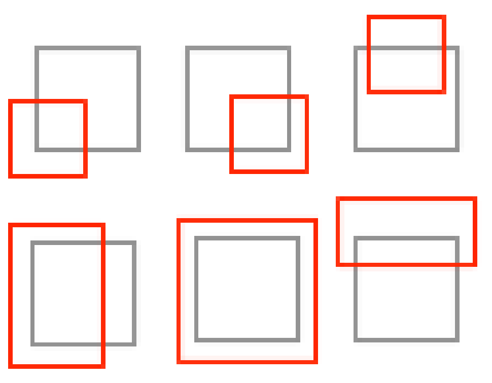
Now we need to function that can determine the types of intersections that could occur between two rectangles (bounds). In the above image, I demonstrate, visually, what these relationships can look like. In the below function, I encode those relationships into vectorized Numpy operations.
def check_if_intersects(row, table):
    # for each point in the bounds, make sure that an intersection
    # can occur at some point

    # check if there are total overlaps with the geometry
    completely_overlapping = (
        (table['bminx'] <= row['bminx']) &
        (table['bmaxx'] >= row['bmaxx']) &
        (table['bminy'] <= row['bminy']) &
        (table['bmaxy'] >= row['bmaxy']))

    # ... repeat for each type of intersection type

    return (total_overlap | bottom_left_is_touching | top_overlaps | all_other_relations | etc)
Now, I can write a function, such as the above, that creates booleans to figure out if at least one of my definitions of what a boundary intersection is exists for each row. This is a completely vectorized operation on Numpy arrays and should be fast as a result. I could further improve performance by using variables to reduce the need to reproduce the same boolean arrays multiple times.
def run_m3():
    possible = gdf3[check_if_intersects(vector_target, gdf3)]
    sub_v2 = possible[possible.intersects(target_geom)]
Regardless, I am now able to update my run an updated subset query that will utilize the vectorized geodataframe’s bounds attributes to return a subset without the use of a spatial index.
The results show that, on a local machine, average performance of this variation clocks it at an average of 0.0269 seconds per run. This is about 5 times slower than when using the spatial index. That said, there are opportunities to utilize parallelization techniques that have been designed to play well with Pandas and Numpy arrays using this method that prior may not have been as easily accomplished. That is to say, parallelizing GeoDataFrame operations is not something that has been developed as a capacity within the Python community as of yet, while parallelization support for Numpy as Pandas is robust. By converting GeoDataFrames to standard Pandas DataFrames with vectorized bounds attributes, we open the door for possible optimizations to the execution infrastructure that may not have been possible prior.
That said, it is worth acknowledging the significant value of the spatial index and to consider it may be worth preserving, if possible, even during parallelization. Here is a notebook if you would like to review the code used in producing this post.
Observing performance as GeoDataFrame size increases
This is an update to the original post as I was curious to see how performance changes as the original GeoDataFrame size increases. We can do this easily by making the base data frame append to itself as many times as we would like to multiply it by. Let’s make it four times larger by appending 4 times (gdf = gdf.append(gdf).append(gdf).append(gdf)). This is sort of sloppy but should work for a quick test. Make sure to reset the index to avoid downstream errors (gdf.reset_index(inplace=True)).
The results are as follows (GeoDataFrame length 119,492):
- Standard, no optimization: 1.86s
- Spatial indexed: 0.005s (+ 9.3µs to create spatial index)
- Vectorized bounds: 0.026s
Again, with a 16x increase (GeoDataFrame length 477,968):
- Standard, no optimization: 7.8s
- Spatial indexed: 0.03s (+ 12.9µs to create spatial index)
- Vectorized bounds: 0.07s
Again, with a 64x increase (GeoDataFrame length 1,911,872):
- Standard, no optimization: 30.75s
- Spatial indexed: 0.045s (+ 21.5µs to create spatial index)
- Vectorized bounds: 0.26s
Again, these sub-second operation times do matter. Imagine doing a row-wise apply operation where the above is essentially performed on each row. One the 120,000 row data frame the spatial indexed version executes in a total time of 600 seconds, or 10 minutes. Meanwhile, the vectorized alternative would clock in at 3,120 seconds, or 52 minutes! These delays only become more severe as the size of the data we are working with gets larger, of course.
Second update: More aggressive curation
It occurred to me that a way to better optimize the check_bounds_intersect() function would be to toss all “definite outliers from the intersection check process before we even enter the helper function itself. To do that, we could toss all items whose furthest extremity lies outside the bounds of the target geometry. Then, once we have those subsetted, we can enter the more detailed check. This would allow us to work with smaller vectors. This should improve performance somewhat.
def run_m4():
    gdf3_temp = gdf3.copy()

    gdf3_temp = gdf3_temp[gdf3_temp['bounds_maxx'] <= vector_target['bounds_minx']]
    gdf3_temp = gdf3_temp[gdf3_temp['bounds_minx'] >= vector_target['bounds_maxx']]

    gdf3_temp = gdf3_temp[gdf3_temp['bounds_miny'] >= vector_target['bounds_maxy']]
    gdf3_temp = gdf3_temp[gdf3_temp['bounds_maxy'] <= vector_target['bounds_miny']]

    possible = gdf3_temp[check_bounds_intersect(vector_target, gdf3_temp)]
    sub_v2 = possible[possible.intersects(target_geom)]
Above is a sketch of how that might work. Here, we simply move the bounds checks for some of the “definite” misses to before we can the check_bounds_intersect operation. Below are there results on a few data frame lengths:
- 29,873 rows: 0.0283s (20.7% speedup vs. orig method: 0.0357s)
- 119,492 rows: 0.036s (16% speedup vs. orig method: 0.0432s)
- 477,968 rows: 0.0829s (37.7% speedup vs. orig method 0.133)
Note: These performance times were calculated by running each operation 25 times and taking the average of the resulting time. This is why times are different than those listed in prior sections. Comparative performance between methods is the primary focus here.
The takeaway from these results would be that such a “tossing” of definite misses prior to the creation of the boolean vector for intersecting bounds helps make this method more competitive when compared with spatial indexing. This likely mimics some of the first steps of a spatial index, which tosses the geometries that lie absolutely outside of the indexed rectangles that intersect with the bounds of the geometry being compared. Still, the the third variation of the above tests (the one that uses 477,968 rows), running the spatial index on this step instead during this series of run throughs resulted in an average performance time of 0.017s, or nearly 5x faster than the optimized vectorized version, still.
Conclusion
Subsequent runs with various improvements on the vectorized alternative to the spatial index seem to continue to solidify the indexes lead as a more performant option when compared with vectorization methods that may simply require too many run throughs of the underlying Numpy arrays to gain from the potential advantages that dealing with just the vectorized column data affords.