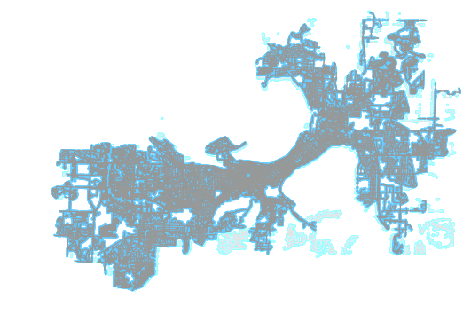
In this blog post, I’ll demonstrate how to clean hanging, disconnected subgraphs as we see in the above image. Lighter areas are dropped and the main network graph (darker portion) is preserved.
Network graphs are the underpinning of many geospatial analytics methods. For example, if you want to know how far away by car and by walk the nearest hospital is to each house/parcel in a city, you might perform the following steps:
- Pull down the OSM ways and nodes from the Overpass API
- Load in an array of all geometries of all parcels in an area
- Load in an array of all points of hospitals in said area
- Attribute the hospitals and parcels to their nearest network nodes
- For each ways in the network, calculate how long it takes to drive and walk it
- For each parcel, traverse network to find nearest hospital and record that time sum by mode (e.g. walk, drive)
By performing the above steps, you could easily create a choropleth map where each parcel geometry is colored from, say, yellow to red. In that map, the more red a parcel is, the longer it would take to walk or drive to the nearest hospital.
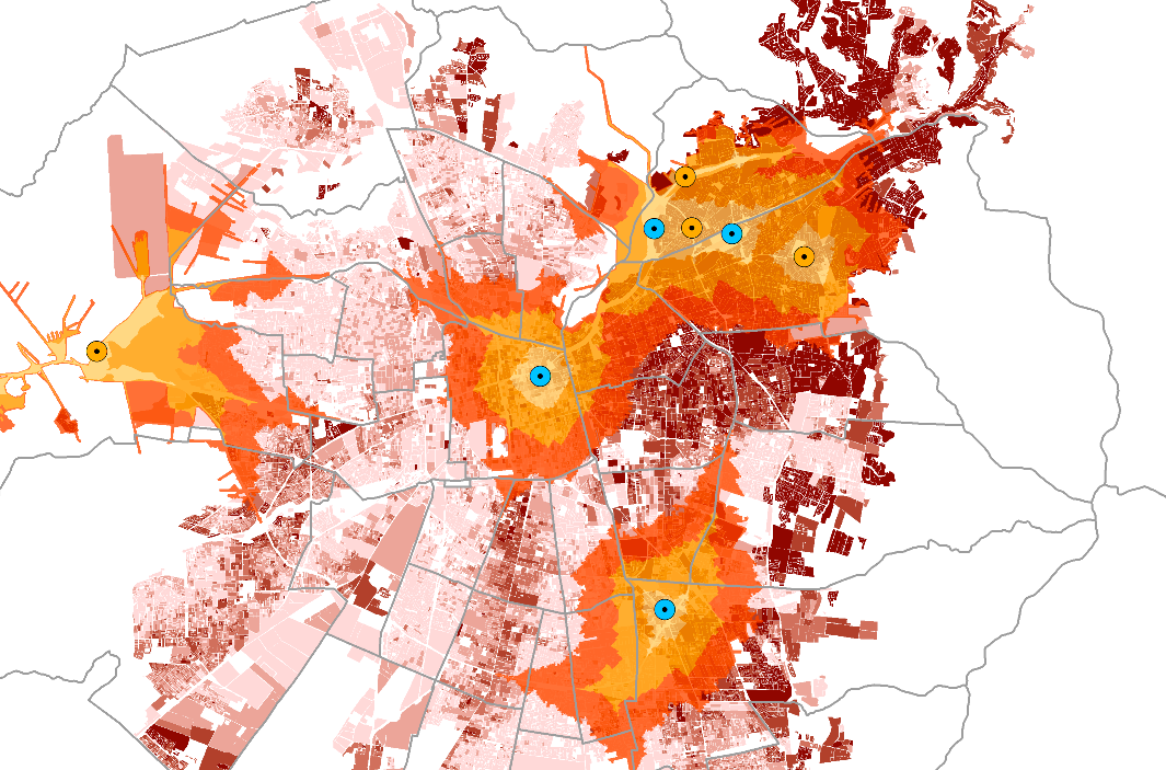
Here’s an example of such a map, by Praveen Subramani. (Who, amusingly, I happen to both know IRL and whose map comes up on Google image search quite quickly.) In this map, accessibility to electric vehicle charge stations is visualized (as opposed to my example of hospitals). You can read more about this project, here.
This is all relatively straightforward but there can be issues that arise when performing this analysis. One such issue is the presence of fragmented networks. When you pull a network down from, say, Open Street Map, you need to ensure that the network you have is connected. Because you might be querying by bounding box, the edges of your bounding box will have network ways that are “frayed.” That is, They will have partial connections sometimes or may be a part of the road network that is disconnected from the rest, within that bounding box you have supplied. Another example might be the capture of a small portion of an area that, within your bounding box, is completely separated by water.
You could imagine a situation such as the bottom of Manhattan which might also return a network portion of Staten Island. More commonly, you might have a small pocket park that has a walk network that has not been connected to the road network. In these cases, for the sake of ensuring successful network analyses at relatively larger scales, it is necessary and defensible to “toss” these smaller networks.
By tossing smaller networks, you can ensure that all geometries are assigned to nearest nodes that are present on the dominant network graph and able to access all other geometries in the network. In this way, geometries avoid becoming “stranded” and unable to access POIs because they remain isolated on a small network graph that exists alongside, but not conjoined to, the main network graph.
Let’s take a look at a real world example. Let’s say we want to look at accessibility measures in downtown Madison, Wisconsin. Let’s query for the whole city of Madison to make sure that we safely buffer the downtown study area.
G = ox.graph_from_bbox(south=south, west=west, north=north, east=east,
                       retain_all=True, truncate_by_edge=True, simplify=False, network_type='walk')
OSMnx is a nice open source tool that can facilitate querying for OSM data and neatly plotting the results. It plays quite well in a Jupyter/iPython notebook, too - I’d recommend it. In the above code snippet, we pull down the OSM network for Madison, Wisconsin.
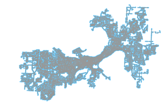
fig, ax = ox.plot_graph(ox.project_graph(G))With the above line, we can have OSMnx plot the network we have pulled down. You can see the resulting output below.
In the output, we can see disconnected networks along the periphery of the network’s plot. For example, in the bottom right there is an O-shaped suburban area that is clearly disconnected from the rest of the network. Harder to see are the myriad of small networks, especially walk networks, that are floating; separate from the overall network. For the purposes of generating useful accessibility analyses, we need to drop these.
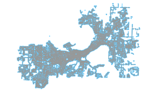
G2 = max(nx.strongly_connected_component_subgraphs(G), key=len)OSMnx is largely based on NetworkX. As a result, we can break apart the network into its component separate subgraphs and identify the largest strongly connected subgraph. A strongly connected graph is one in which all nodes can be reached by all others, whereas a weak one has some nodes which are only accessible one way. If you’d like to read more about weak and strong networks, here’s a helpful Stack Overflow post to get you started.
These “hanging nodes,” from which other nodes can sometimes not be accessed, are largely the typically the product of boundary trims in OSM networks. We could access them, if we desired, by using the comparable NetworkX API call nx.weally_connected_component_subgraphs.
That said, because (in this case) we are pulling down the walk network, each edge is inherently bidirectional (we/OSM does not assume any strict directionality on walk networks, just as you are able to walk either direction on a sidewalk). As a result, all edges between two nodes ought to be represented in both directions. as a result, a query for the largest strongly connected network should be sufficient.
Go ahead and plot this new graph as well. As you can see, the resulting graph has the disconnected issue networks dropped. The two are compared in the image at the top of this post, scroll up top to view the darker preserved area overlaid on the lighter, dropped portions of the network.
Using this new, cleaned network, you are now free to proceed forward with a network analysis of a geospatial layer, by being able to safely attribute each geometry to a node that exists, connected, on a strongly connected single network graph. Happy mapping!