When working on analyses like accessibility, it’s important to properly represent the geometries within the network graph. For example, when working with spatial data against, say, a parcel dataset it is often defensible to use the centroid of each parcel because we are trying to understand that parcel in relation to an entire town, city, or region. In these examples, it is defensible to just use the centroid of the buildings because we are measuring travel over comparatively larger distances. A couple common accessibility measures that might be performed include access to restaurants, schools, and hospitals. These are all fairly common queries (“How far away is the average home or parcel in this area to the nearest emergency room?”).
Why we want to subdivide shapes into points
There are some points of interest that cannot be defensibly represented by a single point of interest. For example, parks a a great example of this. Imagine if Central Park in New York was represented by a single point. All the properties on the north and south side of the park would appear to have far lower accessibility to a nearest park than those on the east and west side of the park
With something like Central Park, a clear path forward can be found by chunking it up into smaller rectangles. If we want to check access to acres of park, we could subdivide the rectangles accordingly. Then each of these smaller geometries could have centroids placed on the network and results would be more accurately mapped onto the network.
An example of a park geometry that is both real and really not a regular shape!
What happens, though, when a geometry is a more complex shape? Sure, we could just arbitrarily break it up into chunks by breaking it up along latitude and longitudinal vertices, but that would not best handle the weird squiggles or branches of complex park shapes. Many parks run along rivers, or wind between housing developments. How do we properly represent those shapes on the network and make sure that neighboring points retain their accessibility measures when mapped on to the network?
Introducing triangulation
The answer lies in the implementation of Delaunay triangulation to subdivide these parks into sub-geometries that properly represent the complexities of the parent shape.
Shapely has a built-in method that triangulates a given polygon. To do so, it simply subdivides the geometry via all it’s nodes, drawing vertices to all other near nodes. The resulting shapes are a series of triangles that map to the original shape. The code for performing this naive triangulation is as follows:
from shapely.ops import triangulate
triangles = MultiPolygon(triangulate(poly))
gpd.GeoSeries([triangles]).plot(figsize=(10,10))
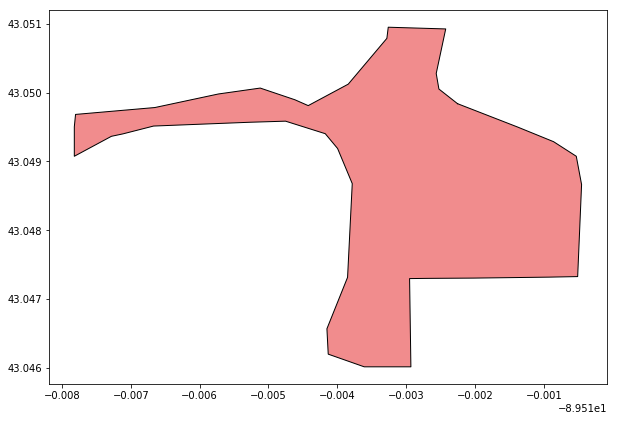
Let’s start with the above shape, from above. This shape has convex components in the bottom left and upper right portions. Were we to apply a simple triangulation method. Let’s apply the naive Shapely triangulation method on that park geometry.
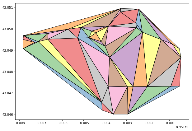
As we can see in the above, the resulting shape is not representative of the original, parent shape. Multiple triangles fall outside of the parent shape. This is because the naive method does not account for the concave aspects of the parent geometry’s envelope.
Background on constrained Delaunay triangulation
It isn’t much more work to run a constrained Delaunay triangulation. There’s a library called (“Triangle”)[https://pypi.python.org/pypi/triangle/20170429] that basically performs the tough part for us. From the Github repo: “Python Triangle is a python wrapper around Jonathan Richard Shewchuk’s two-dimensional quality mesh generator and delaunay triangulator library, available here.”
So, what does the underlying generator do? According to the underlying package’s site: “Triangle generates exact Delaunay triangulations, constrained Delaunay triangulations, conforming Delaunay triangulations, Voronoi diagrams, and high-quality triangular meshes.”
If you are curious to learn more, the Wikipedia page is a good place to start. Basically, through this algorithm, we can break a geometry down into representative triangles of minimum cumulative complexity. Also important is that it does not return “sliver” triangles. As a result, this is a terrific mechanism for getting good, representative triangles along the long “arms” of strangely shaped parks.
Sliver triangles are avoided via the use of threshold. For a given cloud of points, multiple triangulation combinations are possible, but many include sliver triangles. For an example of this, see slide 5 of this presentation. By setting a threshold of a larger angle, say 20 degrees, we can toss resulting triangulation combinations where one or more angles in any of the triangles composing the total triangulated geometry are less than that threshold. By using a larger angle, such as 20 degrees, we can safely ensure that sliver triangles are parsed out of the resulting triangulation.
Note: A special thanks to Geoff Boeing for showing me this methodology! Without him demonstrating this method, I’d likely still be performing some sort of points grid overlay to get representative points from a geometry!
Implementing a constrained Delaunay triangulation
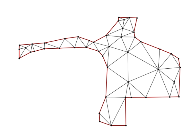
Running the constrained Delaunay triangulation results in a dictionary which describes all vertices and edges (segments), within the dictionary. Using the Triangle library’s helper method tplot, we can see what the new triangle looks like (as in the above image).
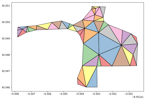
We can now use that dictionary to craft new polygons of each of those triangles, as in the above image.
The representative cloud of centroids now better maps to the original geometry shape (per the above image). This is in contrast to a single point that would have fallen in the middle of the geometry. In this case, we have increased the number of representative points from 1 to 51 points.
Here’s the script used to create that triangle:
# break out coordinates
c = list(poly.exterior.coords)

# and vertices
v = np.array(c)

# and indices
i = list(range(len(c)))

# segments
s = np.array(list(zip(i, i[1:] + [i[0]])))

# 'p': planar straight line graph
# 'q20': indicates triangles need a min angle of 20˚
cndt = triangle.triangulate(tri={'vertices': v, 'segments':s},
                            opts='pq20')
Observe an example geospatially
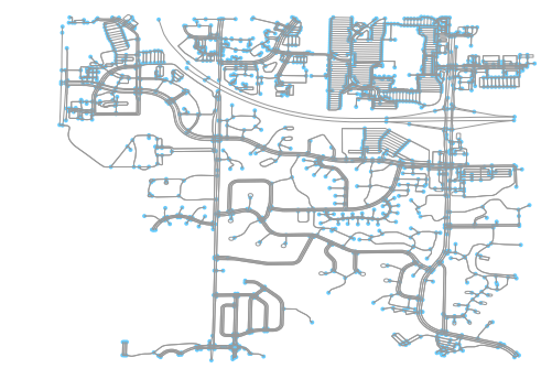
Let’s look at what happens when we place that geometry in a real world setting. First, let’s observe the site that this project is within.
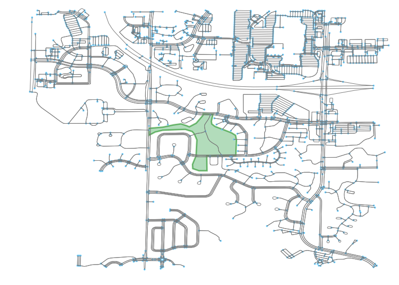
And now we can add the park to that site.
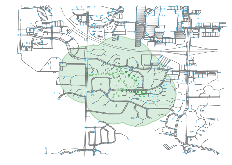
If we buffer that site, we can see the number of points that would fall within “range” as being near this park. Yes, I know the right thing to do here would be to actually use the network to calculate which points have access to the park, but for now I am just going to use spatial buffers as it is more visually clear and gets the point across.
If we just take a single centroid representative point of this park, we can see that we in no way capture the same amount of points. It will look like this neighborhood has far lower accessibility to this park than it indeed does.
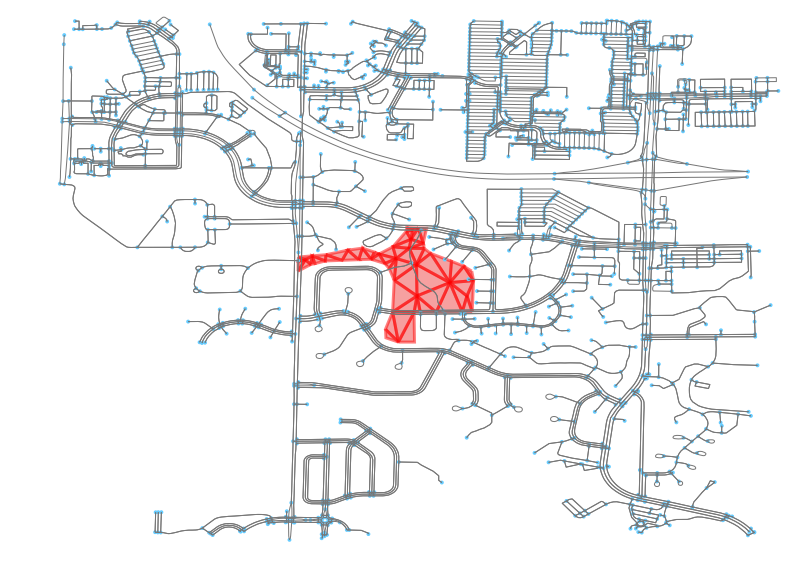
Now let’s triangulate the original park. We can see how it is now composed of the same 51 triangles from earlier.
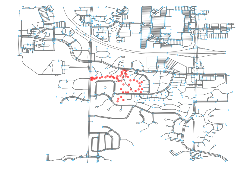
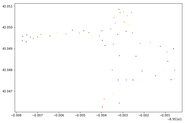
And, again, we can see the result of getting the centroids from each of the triangles. We now have a point cloud of points that “looks” more like the original parent geometry.
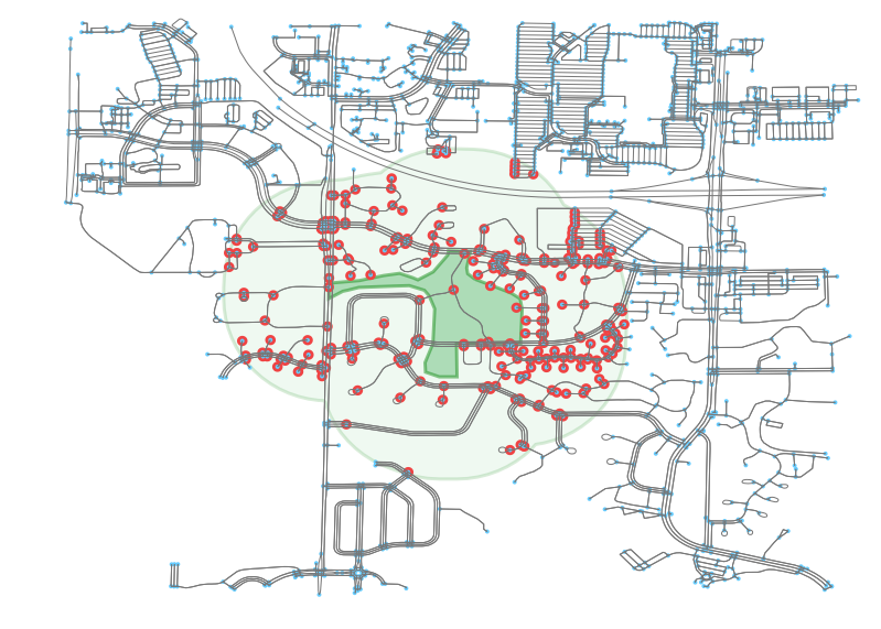
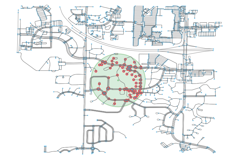
Buffering these points, we end up with a catchment area that far better resembles the original image.
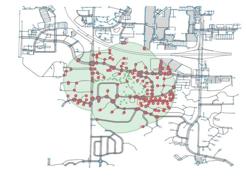
This point is crystalized when we observe the points that fall within the capture area, which is nearly all those from the original geometry buffer.
As was acknowledged earlier, a more correct strategy would be not have buffered the geometry and points, but to have then applied the points to a network graph and crawled that to get access levels. But, for the sake of visualization, this method is sufficient for illustrating the utility of the Delaunay triangulation method in creating better point cloud abstractions of complex geometries.