Note

An updated version of this post, featuring more pictures and better spelling and sentence structure has been posted to Transitland’s blog. You can read it, here, or by clicking the below embedded tweet:

Follow @buttsmeister's tutorial at https://t.co/2kyHQfjmd1 and soon you'll be making your own maps from Transitland using Python + GeoPandas pic.twitter.com/neujX7x350

— Transitland (@transitland) October 25, 2017

Introduction

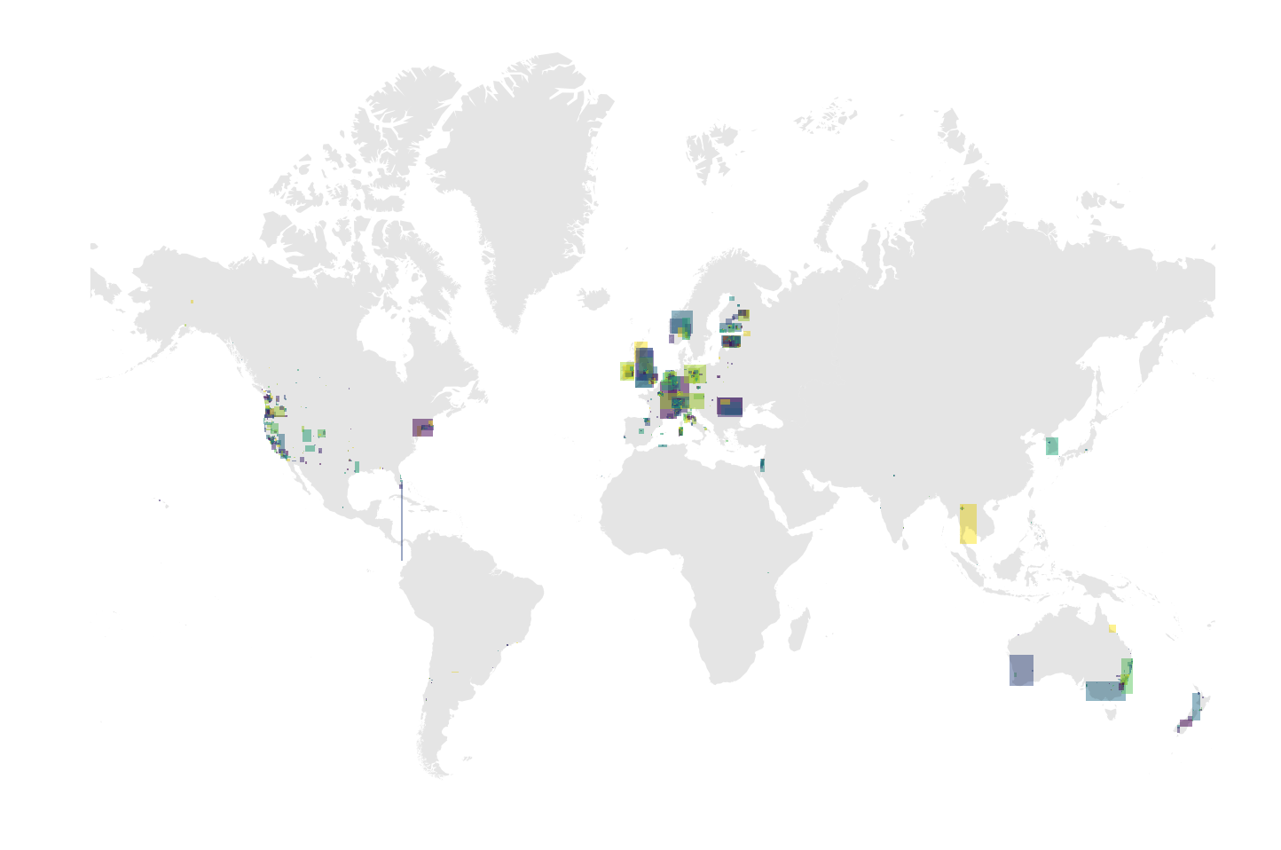
Recently, I posted the above image on Twitter. It generated some positive responses, so I went ahead and generated a few more, one for each continent as well as a few “special requests.” Also included was a script that would allow someone to recreate the same scenes themselves. This post will provide more context around the steps listed out in that notebook, as well as some notes about how tools such as GeoPandas and Shapely can help make the process of exploring Transit.Land’s API more visual and, perhaps, easier to peruse.

Before I continue, I should note that the Transit.Land website already has solid documentation. In particular, the API page has a nice table that explains what each of the possible endpoints are and how the requisite parameter must be formatted. It also includes an example for each.

Setting up a search environment

The focus of this post is to show how one can visually explore the API’s offering by location. In order to do this, let’s find a place with Nominatim. Nominatim is a places dataset that is based on OpenStreetMap data. What we will do is design a simple function to query for a particular place and visualize it on the map. Before we continue, we will should also pull down a shapefile for the continents in the world so that we can plot that as well to see where our target area lies on the map. This will help us sanity check where we are working and make sure that our data is what we think it is.

A simple function (below) will allow us to make queries against the Nominatim API. The parameters passed in will allow us to receive a GeoJSON in response. We can then take that JSON and convert it into a Shapely shape object.

def nominatim_query(query):
    params = OrderedDict()
    params['format'] = 'json'
    params['limit'] = 1
    params['dedupe'] = 0
    params['polygon_geojson'] = 1
    params['q'] = query

    url = 'https://nominatim.openstreetmap.org/search'
    prepared_url = requests.Request('GET', url, params=params).prepare().url

    response = requests.get(url, params=params)
    response_json = response.json()
    return shape(response_json[0]['geojson'])

With the resulting shape, we have the opportunity to easily pass this through to the Transit.Land query.

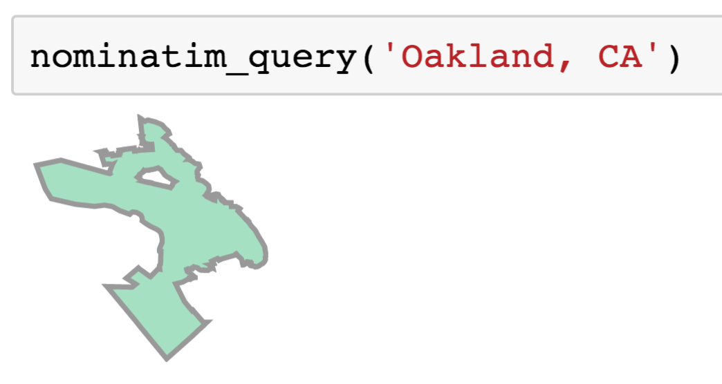
In the above image we can see what the result of running such a query would look like, in this case for Oakland, California.

Preparing the Query into Subcomponents

Using that same helper function we created from the last section, we can now query for the United States the shape of the country. We can pull out the mainland as it is the largest geometry in the MultiPolygon, like so:

all_areas = [u.area for u in usa]
i = all_areas.index(max(all_areas))
mainland = usa[i]

Now that we have the “mainland” area, if you will, we can use Shapely’s API to interact with the shape. To query against Transit.Land’s data, we will need a bounding box. We can get this from the object representing the US mainland: mainland.bounds. The result of this is the following: (-125.0840939, 24.2520071, -66.8854162, 49.3844901).

We can now query Transit.Land for this entire area. In order to ensure that we don’t time out the requests, we’ll need to break this up into a series of numerous, small query. We can design a function to accomplish this recursively as setting limits on the response length in Transit.Land comes with the ability to “pick up where you left off” and query the next n features after the ones you just received. This can be useful for downloading queries from larger areas in small chunks.

Below is a sketch of what such a method might look like:

def recursive_query(target_area=None, full_url=None):
    geoms = []
    names = []
    
    if target_area:
        bbox = ','.join(map(lambda x: str(x), target_area.bounds))
        resp = requests.get(url='https://transit.land/api/v1/operators', params={'bbox': bbox, 'per_page': 50})
    else:
        resp = requests.get(url=full_url)
    resp_json = json.loads(resp.text)
            
    for g in resp_json['operators']:
        geoms.append(shape(g['geometry']))
        names.append(g['name'])
    
    # Check if we should also try and pu
    meta = resp_json['meta']
    if 'next' in meta.keys():
        sub_gdf = recursive_query(full_url=meta['next'])
        geoms = geoms + list(sub_gdf['geometry'].values)
        names = names + list(sub_gdf['names'].values)

    gdf = gpd.GeoDataFrame({'names': names}, geometry=geoms)
    gdf.crs = {'init': 'epsg:4326'}
    
    # Only recast projection on the top level return
    if full_url is None:
        gdf = gdf.to_crs({'init': 'epsg:3857'})
    return gdf

As we can see in the above code, we check if the response JSON contains the key that would indicate that there are more results to be retrieved from the query. We can also see how we introduce the bbox (bounding box) as a query parameter. Simply including that and the per page limit allows us to create a simply function that pulls all results for operators that intersect that area in incremental 50-unit chunks. Only on the final return that exits the top level function do we convert the operator shapes to the meter based projection that we are also going to be using for the continents.

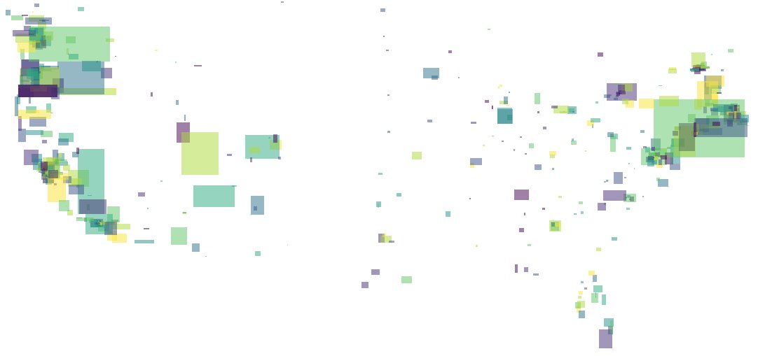
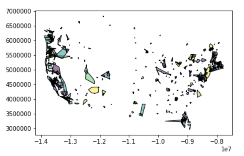
As of the time of this post, there were 606 operators that were returned using the above query. If we plot the resulting GeoDataFrame, we can see that our results include a number of operators that are national in scale. These large operators also include some placeholder shapes that wrap the length or height of the entire projection plane. We should drop these out.

Let’s just go with something arbitrary and check out the results. Let’s say that we want to keep anything that is about 200 by 200 miles. This would be 40,000 square miles. Converting that to square meters (the projection the operators are presently in) would look like this:

cont_sub = all_operators[all_operators.area < 1.036e+11]

Go ahead and plot that result.

What should be visible should look similar to the above. As you can see, results should appear to roughly correlate to the shape of the portion of the United States we are working with. At this point, it would be helpful to have some context. In this case, we can use that “mainland” USA shape from earlier.

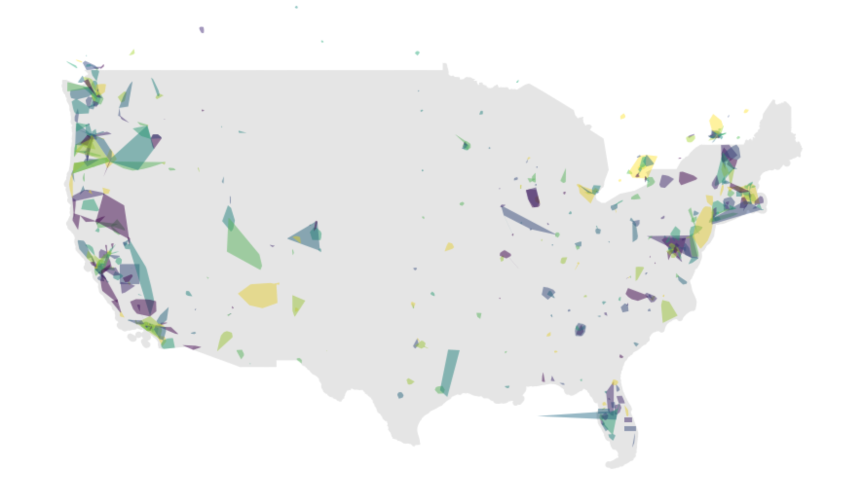
The following script should produce the above image. By passing the ax axis object from one plot operation to the next, we are able to layer plots on top of one another in Matplotlib, such that the resulting image from the two plot operations is a single .png.

ax = cont_sub.plot(figsize=(15,15), cmap='viridis', scheme='quantiles', linewidth=0, alpha=0.5)

mainland_gdf = gpd.GeoDataFrame(geometry=[mainland])
mainland_gdf.crs = {'init': 'epsg:4326'}
mainland_gdf = mainland_gdf.to_crs({'init': 'epsg:3857'})
mainland_gdf.plot(ax=ax, color='k', linewidth=0, alpha=0.1)

As you can see, the shapes are fairly abstract. There shapes correspond to the convex hull, representing an approximate area of coverage for all lines within that transit feed.

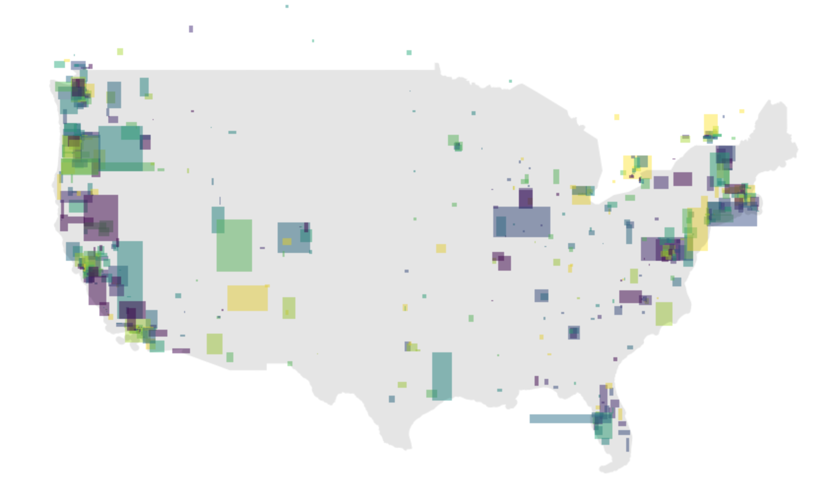
Getting to squares helps make the coverage map more visually clear. To generate this image instead, we simply need to replace each geoemtry with its corresponding bounds. This can be retrieved via the Shapely class’s bounds method.

cont_squares = cont_sub.copy()
cont_squares.geometry = list(map(lambda g: box(*g), cont_sub.bounds.values))
ax = cont_squares.plot(figsize=(15,15), cmap='viridis', scheme='quantiles', linewidth=0, alpha=0.5)
mainland_gdf.plot(ax=ax, color='k', linewidth=0, alpha=0.1)

In the next section, let’s work on pulling down some context layers to use with our operator shapes.

Generating a base layer

When plotting the results, it will be helpful to have a base layer. A base layer in this case might best be the continents of the world. While we did have the “mainland” layer that we used in the prior section, it would be helpful to include the entire world, particularly if we are floating around the map making queries and don’t want to worry whether or not we have the appropriate part of the world already loaded up.

The below function will pull a GeoJSON that is hosted on Github down via the requests library. It loads the response text as a JSON and then pulls out the GeoJSON component. It takes that and loads it in as a GeoDataFrame. You’ll also note that the projection is explicitly stated and updated within the function. It starts being pulled down as EPSG 4326. This is a common, degrees-based projection. We convert it to EPSG 3857, which is a common meter based projection that has coverage over the whole plant. This allows us to think of area and shape perimeter in terms of meters, which will be handy when thinking about the shapes and area of coverage more intuitively.

def make_world_dataframe():
    url = ('https://gist.githubusercontent.com/hrbrmstr/'
           '91ea5cc9474286c72838/raw/59421ff9b268ff0929b051ddafafbeb94a4c1910/'
           'continents.json')
    resp = requests.get(url=url)
    data = json.loads(resp.text)
    
    geoms = []
    names = []
    for f in data['features']:
        s = json.dumps(f['geometry'])
        g1 = geojson.loads(s)
        geoms.append(shape(g1))
        names.append(f['properties']['CONTINENT'])

    gdf = gpd.GeoDataFrame({'name': names}, geometry=geoms)
    gdf.crs = {'init': 'epsg:4326'}

    gdf_proj = gdf.to_crs({'init': 'epsg:3857'})
    
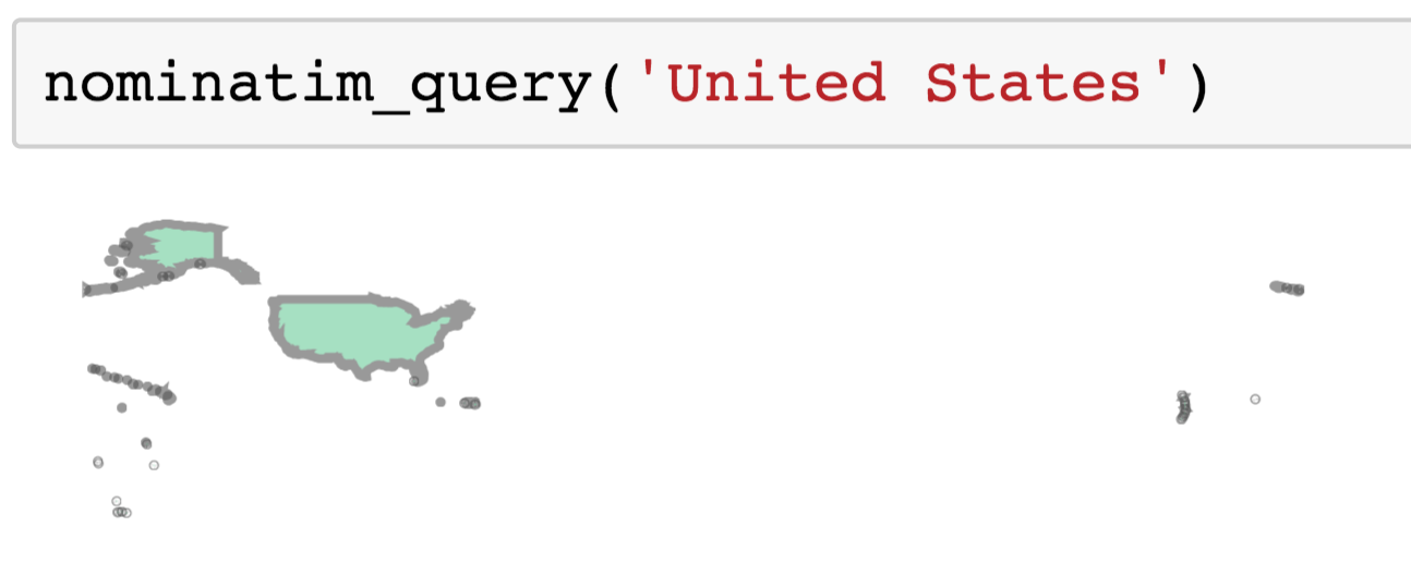
    return gdf_proj

Once we execute this function, we can plot the results to view the countries. The resulting GeoPandas GeoDataFrame behaves similarly to a Pandas DataFrame. In fact, all methods that can be performed on a Pandas DataFrame can be performed on a GeoPandas GeoDataFrame. A GeoPandas GeoDataFrame simply requires a column that holds within it Shapely geometry objects. GeoPandas GeoDataFrames offer a set of methods that allow row-wise operations to be performed on each of those Shapely geometry objects held in the geometry column. In addition to geometry manipulation, there are added plotting capacities on top of Pandas’ that will enable plotting of spatial information.

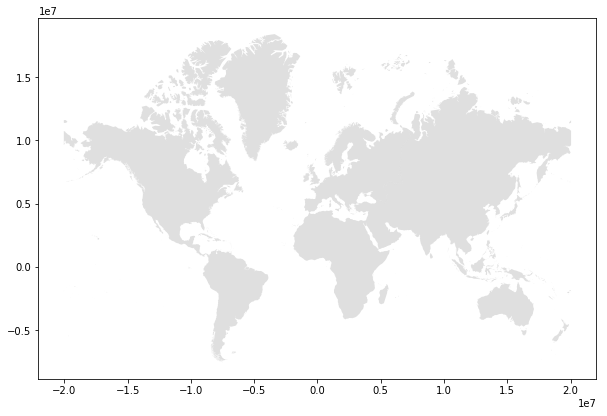
The below code uses the GeoDataFrame’s plotting functionality and will plot all continents (save for Antartica, which is queried out). The output of this function is visible in the above image. If working in a Jupyter Notebook, make sure that the inline plotting setting is added by including %matplotlib inline at the top of your notebook.

world_gdf = make_world_dataframe()
without_ant = world_gdf[~(world_gdf.name == 'Antarctica')]
without_ant.plot(figsize=(10,10), color='grey', linewidth=0, alpha=0.25)

Using the base layer we generated, we can easily move to new parts of the world. We can generate plots on subsets of total continents by breaking down the MultiPolygons of each continent. We can do so by iterating through each, so that we only deal with single Polygons at a time, like so:

# Break each element of each continent into a separate
# Polygon so that we do not have to select a single 
# continent in its entirete
clean_gs = []
paired_names = []
for i, row in world_gdf.iterrows():
    name = row['names']
    for g in row['geometry']:
        clean_gs.append(g)
        paired_names.append(name)

con_expl = gpd.GeoDataFrame({'names': paired_names}, geometry=clean_gs)

Exploring new areas

With out broken down continents layer, we can now draw new subsets of the world on a map. Let’s go to GeoJSON.io, for example, and draw a rough border around New Zealand and Australia. Using the draw functionality on this page, it should be easy to draw a rough polygon around these two countries. Once we have that, go ahead and cut and paste that shape from the right hand side GeoJSON string. It should look like this:

aus_nz = {  "type": "Polygon",
            "coordinates": [
                [ [ 137.900390625, -11.436955216143177 ], 
                  [ 129.0234375, -8.407168163601076 ],
                  [ 115.83984375, -15.538375926292048 ],
                  [ 109.951171875, -27.68352808378776 ],
                  [ 115.04882812499999, -39.09596293630548 ],
                  [ 142.822265625, -47.4578085307503 ],
                  [ 166.2890625, -48.400032496106846 ],
                  [ 175.693359375, -40.84706035607121 ],
                  [ 178.41796874999997, -37.64903402157864 ],
                  [ 171.826171875, -33.21111647241684 ],
                  [ 143.08593749999997, -9.535748998133615 ],
                  [ 137.900390625, -11.436955216143177 ] ]
            ]}

With this result, we should be able to intersect that cleaned continents layer and keep only the areas that we want that are relevant to the countries of interest. With this subset, we can perform the recursive Transit.Land search to get all Transit.Land operators that lie within those bounds as well.

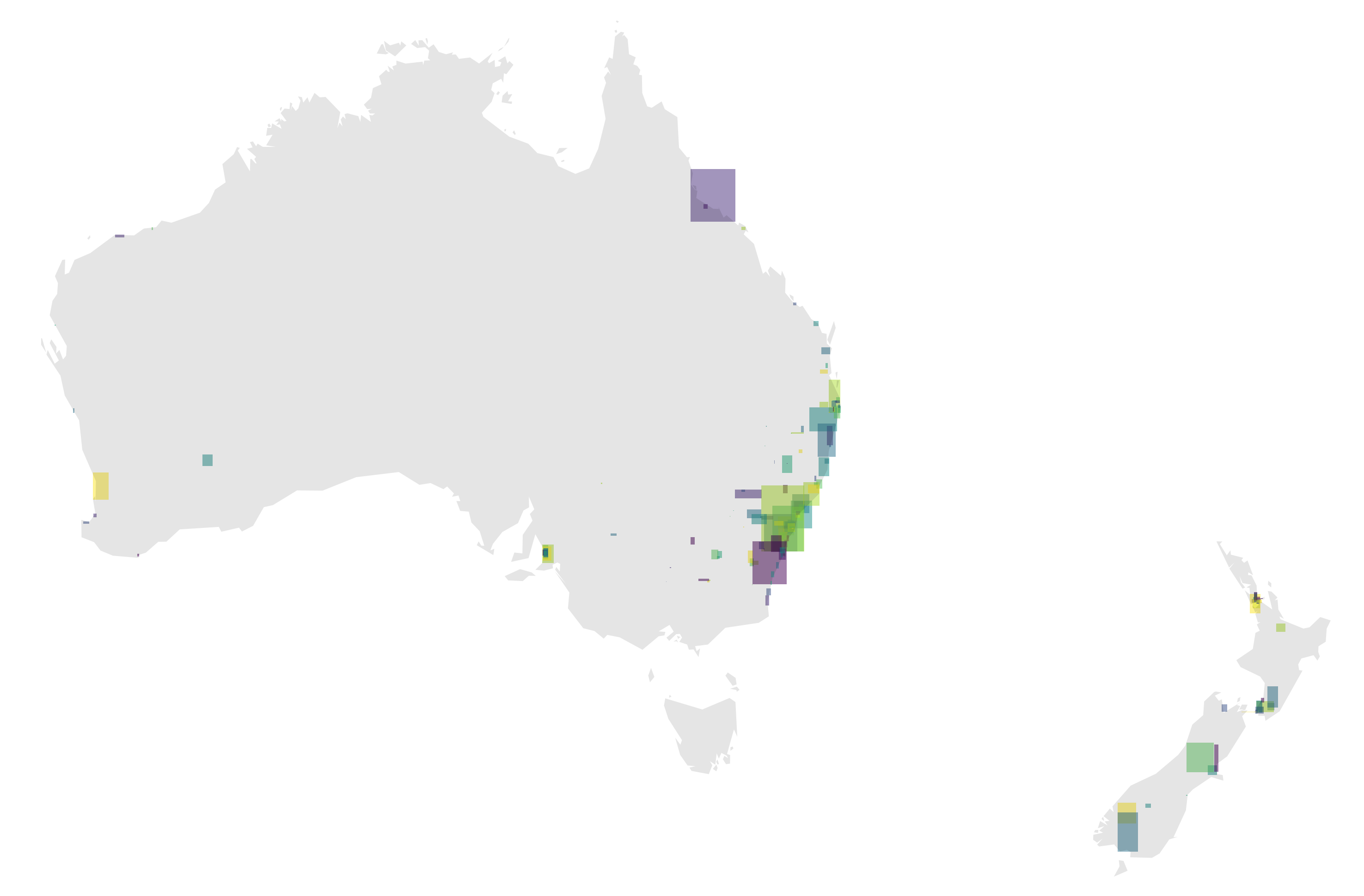
Merging the two should result in the above image.

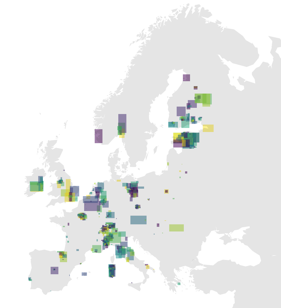
Above, another plot, this time of Europe and western Russia. As you can see, this pattern is easily reproducible anywhere.

Conclusion

At this point you should be free to explore the feeds available on Transit.Land - there’s a ton of them! Need ideas for what to explore next? How about choosing a more refined base layer if you’d like to work at a “closer” scale and explore and work with transit bounds data at, for example, the county and census tract scale in the United States.

Once you find a feed you like, you can download the zip file by examining the url attribute in the API response for a given operator. If given permission, Transit.Land will also hold a copy of the GTFS zip file themselves on an S3 bucket. Simply going to that link will enable you to download the zip file. Once you have downloaded the zip file, there’s plenty of tools out there to explore the schedule data with.

If you enjoy working with Pandas DataFrames and find this data structure convenient when working with ordered datasets such as GTFS (I do!), then you may enjoy Partidge. This is a new but promising library that proposes a standard for how one might organize transit schedule data on a series of Pandas DataFrames, reflecting the same files that would exist in .txt format within the zip file.