Introduction

Recently, my roommate Ben and I have been on a plotting binge. We’ve got our hands on an old, beat up Roland DPX-2000 pen plotter - it’s totally rad! Here’s a video of the same model as ours in action, from about 5 years ago.

Ben has developed a script that takes point array data and converts it to HPGL (Hewlett-Packard Graphics Language), which is then packaged up and streamed to the plotter, which executes the commands. If you are interested in how this is done, feel free to check out Chiplotle. This tool created Python extensions to HPGL plotter control language. Critically, “Chiplotle also provides direct control of your HPGL-aware hardware via a standard usb<->serial port interface” (source: PyPI)

Through this conversion script, we’ve been able to make some interesting plots. Naturally, I wanted to take down OpenStreetMap data and plot that, as well.

Below is video footage from this summer, when I attempted to plot Bogota, Colombia:

1/3 done pen plotting a map of the informal transit route splines of Bogota from last weekend. ~8 hrs to go! pic.twitter.com/KAgjDSVBnm

— Kuan Butts (@buttsmeister) September 11, 2017

(Note: You may have noticed a grid like nature to the above plot. This was achieved by running custom joins in Rhino before feeding out the geometries. This was inefficient and I want to not have to do any manual post process of the geometry data for future runs.)

Problem

The result was great, as you can see below. The only problem was that this print operation took the better part of a day to execute

Base done, red transit routes up next (when red pens arrive in mail!). Total time: ~15 hrs. pic.twitter.com/gyRzMVHVJA

— Kuan Butts (@buttsmeister) September 11, 2017

Naturally, this is not acceptable: First, our machine is crazy old, so any additional run time by the machine puts it that much closer to death. Second, longer operations are typically the cause of lots of back and forth and repeated lines being drawn over themselves. These damage the pens we are using and risk us running out of ink during a run. Because our machine is very much jerry rigged, we are unable to stop it mid process or otherwise do anything that would be able to account for having to swap pens mid-run. Third, it just takes too long! It’d be better if the prints were done faster.

Issues with the data

Why do we end up drawing repeated lines? For a number of reasons. There are many edges between any two nodes in OSM and, not only could they be close and, therefore, similar, but they could also multidirectional. As a result, we end up creating edge lines that represent the path for both directions, thus creating the need to draw the same line twice. Removing this alone would, approximately, reduce the run time in half.

Action shot pic.twitter.com/nNwcDRRSES

— Kuan Butts (@buttsmeister) December 5, 2017

This thought came to mind earlier this week when we were running plots of vector terrain data from San Francisco’s open data portal (as seen above).

Unlike vector data, OSM data was different. We were actually working with a series of discrete edges, that were themselves actually only node pairs. Unlike the contour geometries, we did not already have reasonable groupings.

A site

I am trying to prepare a plot of the Cambridge/Boston area. The below image is what the result should look like.

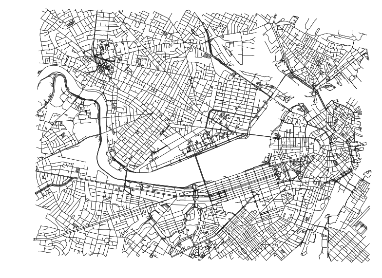
This plot is generated from the edge data pulled down from OSM. A single line is drawn from each from node to each to node. The paths are cleaned, as well as intersections, using OSMnx.

If I were to try and plot the simple result of all edges as generated through this method, I would have the aforementioned issues. Each edge would still be drawn over at least twice, once in each direction. Each edge would also be drawn one small segment at a time. Because the edges are not ordered in any way, the machine would have to stop, lift the pen up, and move to the next tiny line to draw. This is horribly inefficient. The machine’s act of lifting a pen and moving to the next place to drop the pen down is very expensive. As a result, combining as many edges as possible into one long “run” is critical to succeeding. Also, in doing so, there is no stopping at each node so you don’t get fat dots where the plotter stops and also re-drops the pen at every “kink” in the line. This all helps make the map not only finish faster, but look better (more clean, legible).

Idea for how to tackle problem

What we have with the OSM data is effectively a network graph (heck, that is what it is!). We can treat this, devoid of geometries by simply identifying the from and to nodes. What we need is a strategy that effectively mimics a depth first search algorithm.

We want to generate a lot of really long lines. These can be created by finding on node pair, then looking at the “to” node in that pair and finding the next pair whose “from” node matches the previous’ “to” pair. In the depth first version of this, we would continue until we have exhausted all new options and then randomly pick another node to work with.

Indeed, a breadth first approach may be valid as well. In this, we could end up with maybe not a few very long geometries, but at least most would be reasonable long and we would do well in keeping the “orphaned” one-node-pair edges to a minimum.

Frankly, in this case, either will suffice. I opt for depth first.

The code

First, everything you need to do this:

import osmnx as ox
# Make sure to turn this on if you are in a notebook
%matplotlib inline
ox.config(log_file=True, log_console=True, use_cache=True)

import geopandas as gpd
import pandas as pd
from shapely.geometry import box, LineString, MultiLineString

Now, let’s download the network. We can use a metro extract from Mapzen or load in from Overpass API via OSMnx. Whatever works. In this case, I will use OSMnx.

p = box(-71.134501,42.336342,-71.046095,42.385937)
G = ox.graph_from_polygon(p, name='cama', network_type=‘walk')

I also retroject the graph so it’ll look less distorted during the plot (G_proj = ox.project_graph(G)).

Once we have the graph as a NetworkX graph (‘G’), then it is really easy to get the edges dataframe.

def make_edges_df(G):
    dfe = ox.save_load.graph_to_gdfs(G, nodes=False, fill_edge_geometry=True)
    dfe = dfe.rename(columns={'u': 'from', 'v': 'to'})
    return dfe[['from', 'to', ‘geometry']]

We can view that data frame like so:

dfe = make_edges_df(G)
dfe.head()

Go nuts. Most importantly, though, let’s visualize it to see how fragmented it is.

ax = gpd.GeoSeries(dfe.geometry).plot(
    linewidth=0.5,
    cmap='prism',
    figsize=(15,10))
ax.set_axis_off()

The above will generate the below graph.

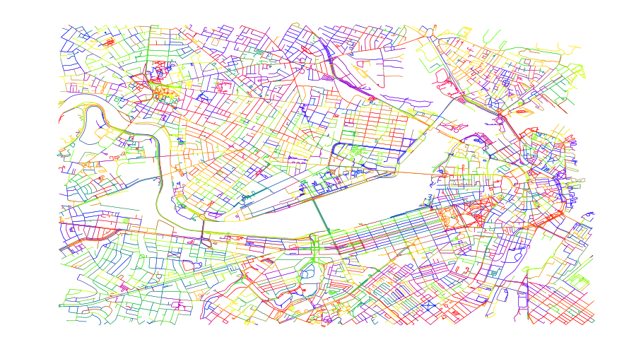
This should help illustrate how disperse all the edges are. Just by the nature of the random color variation, we can see that the plotter is going to be drawing lots of small short lines and jumping back and forth across the plotting area.

If we examine the length of this edge dataframe, we will see it is about 28564 edges. That’s a lot of individual action. Between the lifting and dropping, each edge takes about 1.5 seconds. That’s nearly 12 hours to do a relatively simple plot (we are pretty zoomed into Boston and the Charles river takes about about 20% of the plot). Not good. Let’s reduce the number of unique edges.

Now, before I continue, I am well aware there is a recursive solution here. That said, we’re looking for a good enough solution and this is it.

The below function ignore the geometries and performs the depth first node pairing operation previously discussed. It starts with a node pair and finds the next node pair whose from node pairs with the prior’s to node. It continues until it runs out of possibilities then picks another node.

all_used_ref is a more performant way in Python to keep track of node pairings used than a list of nodes, so we use that to keep track of node pairs. Note that when we find a pair, we tag it in the lookup table for both directions. This keeps us from creating those repeat lines that were brought up earlier, and immediately enable the draw time to be halved.

froms = dfe['from'].values
tos = dfe['to'].values
joined = list(zip(froms, tos))

# Create a ref dict
all_used_ref = {}
for f in froms:
    all_used_ref[f] = {}
for f, t in joined:
    all_used_ref[f][t] = False

assembled_lines = []

for next_pair in joined:
    target_fr, target_to = next_pair

    # First check if we have already assigned this edge
    # and if we have then skip
    if all_used_ref[target_fr][target_to]:
        continue
    # And check for the other direction as well,
    # we treat all edges as undirected
    if all_used_ref[target_to][target_fr]:
        continue

    # Initialize reference values
    keep_running = True
    new_line = [next_pair]

    while keep_running:
        # Default to nothing having happened
        something_happened_this_round = False
        # Get the last element from the new_line tally
        last_fr, last_to = new_line[len(new_line) - 1]
        # Iterate through all joined again, examining
        # each pair
        for fr, to in joined:
            proposed = (fr, to)

            # Skip if this pattern is already in the line options
            if all_used_ref[fr][to]:
                continue
            # Also skip if this is already in the new_line
            # tally, so as to avoid circles
            if proposed in new_line:
                continue

            if last_to == fr:
                new_line.append(proposed)
                # Only allow the running to keep happening
                # if we actually add to the line being assembed
                something_happened_this_round = True
                break

        # Check state of while loop
        keep_running = something_happened_this_round
        
    # Update the all used pairs running tally
    assembled_lines.append(new_line)
    # Update the lookup reference table
    for p_fr, p_to in new_line:
        all_used_ref[p_fr][p_to] = True
        # Do so for both directions (we only do one way)
        all_used_ref[p_to][p_fr] = True

If you were to print the resulting len(assembled_lines), you’d see we reduced the unique edges down to 3,500 edges. That is an 87.75% reduction in length! I’m happy with that. This will work to plot!

Since this is spaghetti code, I opted to sanity check the results - it passed. We don’t have any invalid lines resulting based on the below check. All nodes lead to the next node for each discrete line list of nodes.

# Make sure that all results are
# valid continuous edge pairs
for al in assembled_lines:
    prev_e = al[0]
    for e in al[1:]:
        assert e[0] == prev_e[1]
        prev_e = e

Great, now we should visually check out results. Let’s load up those geometries. Not only will we visually check out results, but our new geometries will be able to be those that are fed into the plotter.

all_new_geoms = []
all_froms = []
all_tos = []
for assembled_line in assembled_lines:
    line_geoms = []
    for tpl in assembled_line:
        fr_n = tpl[0]
        to_n = tpl[1]
        
        # Get subset with from node
        mask_a = (dfe['from']==fr_n)
        df_sub = dfe[mask_a]

        # Get subset with to node
        mask_b = (df_sub['to']==to_n)
        df_sub = df_sub[mask_b]

        # There can be cases where more than one road
        # go to and from same nodepair but we hope these are
        # small details and accept they may be lost
        
        # Pull out one row as Series
        row = df_sub.head(1).squeeze()
        # And add to the line
        cs = row.geometry.coords.xy
        for x, y in zip(*cs):
            line_geoms.append((x,y))

    first_fr = assembled_line[0][0]
    last_to = assembled_line[len(assembled_line)-1][0]
    
    all_froms.append(first_fr)
    all_tos.append(last_to)
    newg = LineString([list(n) for n in line_geoms])
    newg = newg.simplify(0)
    all_new_geoms.append(newg)
    
res_df = pd.DataFrame({'from': all_froms,
                       'to': all_tos})
res_gdf = gpd.GeoDataFrame(res_df, geometry=all_new_geoms)

Note from the above this line: newg = newg.simplify(0). This is important. I actually discovered this method while browsing the old (and, I believe, now defunct) GIS Python mailing list archives. You can find this observation, here. What the author noted was that using the simplify function with a 0 target had the effect of removing repeating nodes. This is important because all of our edges inherently have repeated points throughout due to the way in which they were created. We need to remove that middle point and the simplify step allows us to do that out of Python and instead via GEOS. This is faster and more efficient that iterating over the object through Shapely.

Results

Just like earlier, we can plot the results easily:

ax = res_gdf.geometry.plot(
    linewidth=0.5,
    cmap='prism',
    figsize=(15,10))
ax.set_axis_off()

And, below, the resulting plot:

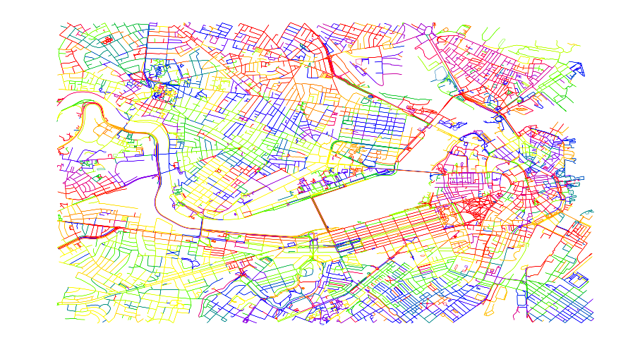
As you can see from the plot, we now have visual color clusters within the map. Not only are lines grouped more so now than before, but the next line typically starts near the previous one (hence how regions end up being the same cluster). This allows the plotter to not have to travel far between plotting lines, which plays a significant role in helping speed up the run.

Using my same 1.5 second estimate from before, this plot will now take only 1.45 hours, down from nearly 12 originally. Well worth the time and effort!