Introduction

The motivation for this post is based on conversations regarding variation in peak hour service. While peak hour is typically defined as some hour range in the AM and PM that roughly corresponds with when most white collar jobs start and end, it is not necessarily peak hour for other sectors and the neighborhoods where those workers are clustered. One way to observe these variations is to look at GTFS data and observe when peak hours tend to occur throughout the day, as defined by some set of constraints. In this post, I set about doing just that, and then attempt to find all hours of the day at each stop in a system where the constraints are satisfied to find out how many hours of peak service it receives, and at what time of day.

This post is intended to be a technical overview of the algorithms designed to extract peak stop hours data at a per-stop level in a given operator’s transit feed (GTFS). A specific example case using SFMTA’s GTFS zip file from late 2017 is forthcoming (it should be posted soon after this post goes up).

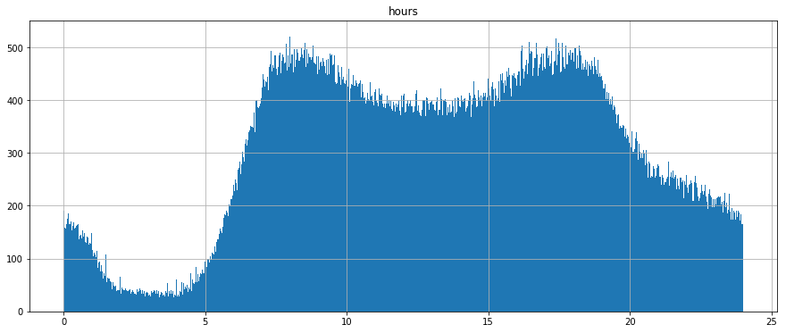
The above plot shows a histogram of the distribuion of all arrival times, system wide, throughout the day. The system being evaluated is SFMTA’s. The data clearly shows a “traditional” AM and PM peak period. That said, not all route services are designed to provide peak service during those time frame.

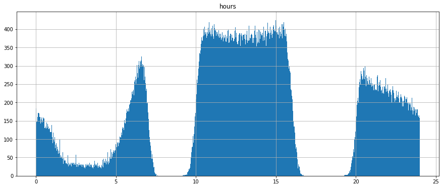
In this second plot, I show another histogram of service arrival times systemwide, bucketed into arrival times by minute. Unlike the prior plot, in this plot I parse out all trips during which the peak service period is within the 2 peak times (7 - 10 AM and 4 - 7 PM - ish) of the overall histogram distribution. The resulting second plot is thus a distribution of service levels at all stops on all trips that provide more service off of main peak than on pain peak. As you can see, there still remains a natural noon-day peak, but there also remains an opportunity for some of these trips to be provided service at stops with “peak period level service” at stops that would otherwise not be counted if I were to only check service levels at each stop during some statically defined peak period.

With the following methodology, I hope to set forth a method of how to identify peak period service level windows. In a subsequent post, I will apply this methodology to a test site (SFMTA), and evaluate the results.

Update

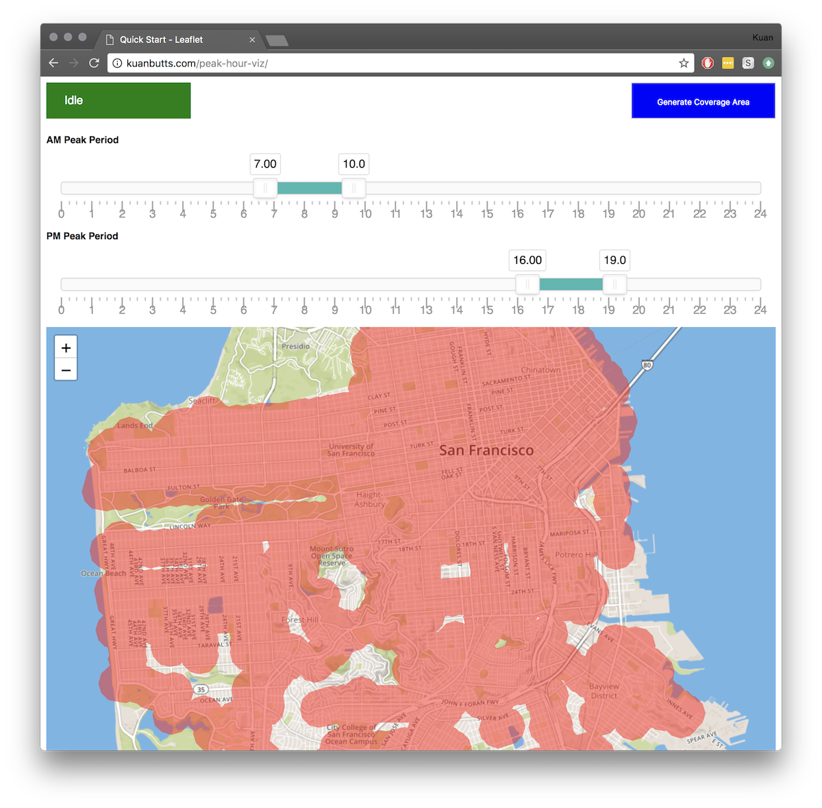
I am not going to do a second post, I will just add some comments to this simple static site that provides some subsetting query tools over the resulting GeoJSON that is created. You can view it here.

Tools and set up

I’ll be using Partridge to map a representative peak service day from a GTFS zip file into a series of data frames. I wrote a method in Peartree that takes a given feed and finds the service ID with the highest number of trips. This reliably maps to a typical busy weekday schedule. From this subset, I will tease out when peak services, as defined by a series of constrains, occurs for each stop in the system.

This method has been adapted and also exists in Partridge, so there is now no need to include Peartree if you have a more recent version of Partridge.

At any rate, these are the libraries utilized in the following exercise:

import json
import math
import os
import sys
from typing import Dict, List

import geopandas as gpd
import networkx as nx
import pandas as pd
import partridge as ptg
import peartree as pt

Caveats

I do acknowledge a limitation in the utilization of this representative feed output. Because I ultimately end up picking one service ID to work with, I do risk missing regular peak service in areas that don’t run service on traditional busy days. On the other hand, accounting for such situations would also necessitate parsing out special event schedule and similar such schedules, which itself is a rabbit hole I am opting to not go down for now.

Assumptions and global defaults

I will be setting some global thresholds that will be used later on in the various functions. The are listed, below:

# Global defaults
BUFFER_DISTANCE = 76.2  # about 250 feet in meters
ONE_HOUR = (60 * 60)  # time in seconds
BUS_ARRIVALS_PER_HOUR_THRESHOLD = 8
BUS_ROUTE_COUNT_THRESHOLD = 2  # must have >= this value to be considered HQT

Buffer distance is the distance, in meters, that I use to cluster bus stops together. For the purposes of frequency assessment, all bus stops within that set distance of a target bus stop being evaluated are considered approximately the same and thus all arrivals to all bus stops within range are deemed part of the same and thus contribute to it likely being a high quality transit (HQT) stop.

Bus arrivals per hour is an alternative to the 15 minute headway definition of a HQT corridor. Instead of caring about the headway distribution, I want to make sure that, over a given hour of the day, starting at any second of the day and going for exactly one hour, there are at least 8 arrivals to that given bus stop (and its neighboring paired stops).

Similarly, the bus route threshold is used to trim results further by saying that, for this given bus stop cluster, there need to be a certain number of discrete/unique bus routes composing those 8 or more arrivals for it to be considered HQT. In this case, it has been set to 2. That means I need these stops to be being serviced by at least 2 routes in that given window of time.

Primary objects data classes being developed

I will work with two data classes in this operation. Each will represent a different key component of the processed data. First is the StopHourWindow:

class StopHourWindow:
    def __init__(self,
                 start: int,
                 end: int,
                 arrival_count: int,
                 route_count: int):
        self.start = start
        self.end = end
        self.arrivals = arrival_count
        self.routes = route_count

The StopHourWindow is intended to represent a calculated window of time around a stop and the number of arrivals that are computed to occur during that window. The start and end times are calculated by adding 30 minutes before and after the arrival time of in the schedule feed to get a 60-minute window of time with which to assess the schedule data.

The arrivals attribute represents a count of all arrivals that do occur in that hour time window and the routes count is an integer representing how many unique routes are paired with those arrivals.

One level up from the StopHourWindow is the StopPeakTimes:

class StopPeakTimes:
    def __init__(self,
                 count: int,
                 windows: [StopHourWindow],
                 lon: int = None,
                 lat: int = None):
        self.count = count
        self.windows = windows
        self.hours = len(windows)

        # Location only added if the values
        # are both supplied
        self.location = None
        if lon and lat:
            self.location = (lon, lat)

StopPeakTimes represents a summary of the number of discrete hour periods that satisfy all constraints. From this, the total number of hours of the day that have peak service, as defined, is summed. Other information is also preserved to help uniquely identify and site the stop.

Walkthrough

At a very high level, I simply read the data in:

feed = pt.get_representative_feed(‘data/sfmta.zip')

Then, I create a cross walk of all other stops that lie within the set distance threshold for clustering stops with each given stop:

stop_pairs_xwalk = generate_stop_pairs(feed.stops, BUFFER_DISTANCE)

Next, I iterate through each set of keys and get compute the number of hour windows in the day that satisfy the constraints set for a peak hour:

stop_peak_times_lookup = {}

all_keys = list(stop_pairs_xwalk.keys())
for i, key in enumerate(all_keys):
    print('On {}/{}...'.format(i + 1, len(all_keys)))
    try:
        # Extract all possible times that satisfy 8
        # arrivals per hour
        valid_periods = get_valid_periods_for_stop(
            stop_pairs_xwalk, key, feed)

        # Then get best set of hours that satisfy
        # the arrival and min-route-count contraints
        optimal_hours = get_optimal_hours(valid_periods,
                                          BUS_ROUTE_COUNT_THRESHOLD)

        # Skip any stop id that has no possible hour windows
        if not optimal_hours:
            continue

        # Add to the lookup dictionary
        optimal_hours.location = get_stop_coords(feed.stops, key)
        stop_peak_times_lookup[key] = optimal_hours
    
    # If an error occurs, make a note of it and go to the next
    # stop to evaluate
    except Exception as e:
        print('\tError occured: {}'.format(e))
        continue

We can observe the results of the optimization step via the following two plots:

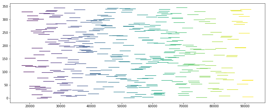
Or, if we were to sort all those windows in order of ascending start time:

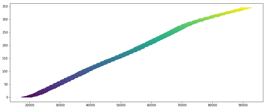
The first shows all valid windows for a given stop. As you can see, there is a significant amount of overlap as many arrival times are associated with valid window periods that satisfy the set costraints supplied.

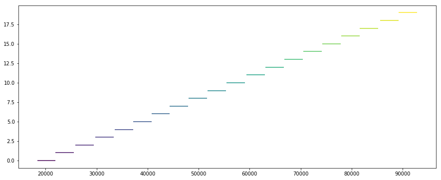
Via the recusive job sorting optimization function, I am able to perform a modified “bin-packing-esque” operation that acheives the goal of applying (or, rather, fitting) the maximum number of valid hours into the set 24 hour period.

Note, the above plots are generated simply:

valid_periods = get_valid_periods_for_stop(
    stop_pairs_xwalk, key, feed)

all_windows = []
for w in valid_periods:
    all_windows.append([w.start, w.end])

df = pd.DataFrame(all_windows, columns=['start', 'end'])

minv = df.start.min()
maxv = df.start.max()

color_vals = []
cmap = plt.get_cmap('viridis')
for s in df.start:
    pct = ((s - minv) / (maxv - minv))
    color_vals.append(cmap(pct))

plt.figure(figsize=(15,6))
plt.hlines(df.index,
           df.start,
           df.end,
           colors=color_vals)

Similarly, the optimal hour windows plot is generate be replacing the valid_periods object instead with the optimal_hours iterable object.

Finally, I export the results as a GeoJSON:

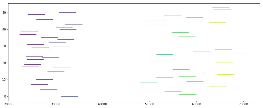
convert_to_geojson(stop_peak_times_lookup)

Here’s another plot, this time with a more typical stop, that has a clear AM and PM peak:

Details on function

All functions are included below, fully fleshed out. Details are added beneath each as applicable.

This first method is used to create the stop clusters based on the maximum threshold distance that has been set in the global parameters.

def generate_stop_pairs(stops_df, buffer):
    all_stops_paired = {}
    all_stops_lat = stops_df.stop_lat
    all_stops_lon = stops_df.stop_lon
    for i, stop_row in stops_df.iterrows():
        lat1 = stop_row.stop_lat
        lon1 = stop_row.stop_lon
        distances = pt.toolkit.great_circle_vec(lat1,
                                                lon1,
                                                all_stops_lat,
                                                all_stops_lon)
        mask = (distances <= buffer)
        stops_ids_within = stops_df[mask].stop_id.tolist()
        all_stops_paired[stop_row.stop_id] = stops_ids_within
    
    return all_stops_paired

The below method goes through each possible stop time and takes a 30 minute window on either end of its arrival time. From that window, it sees how many other arrivals are occurring in that timeframe. It tallies that up and, if it satisfies the arrival threshold, it also then calculates the number of unique routes involved. It places all of this information in an object and returns a list of them when the function is done.

def get_valid_periods_for_stop(
        stop_pairs_xwalk: Dict[str, List[str]],
        key: str,
        feed: ptg.feed) -> List[StopHourWindow]:
    stop_ids = stop_pairs_xwalk[key]
    stop_ids.append(key)

    st_times = feed.stop_times
    trips_df = feed.trips

    st_times = st_times[st_times.stop_id.isin(stop_ids)]
    st_times = st_times[~st_times.arrival_time.isnull()]
    st_times = st_times[~st_times.departure_time.isnull()]
    st_times = st_times.sort_values(['arrival_time'])

    valid_periods = []
    for arr_time in st_times.arrival_time:
        window_start = arr_time - (ONE_HOUR / 2)
        window_end = arr_time + (ONE_HOUR / 2)

        st_sub = st_times[st_times.arrival_time >= window_start]
        st_sub = st_sub[st_sub.arrival_time < window_end]

        trip_ids = st_sub.trip_id.unique()
        bus_arrival_count = len(trip_ids)

        # I can create a potential hour period that
        # satisfies the constraint if this is passed
        if bus_arrival_count > BUS_ARRIVALS_PER_HOUR_THRESHOLD:
            # I need to get the number of unique bus stops, too
            trips_sub = trips_df[trips_df.trip_id.isin(trip_ids)]
            route_ids = trips_sub.route_id.unique()
            unique_routes = len(route_ids)

            # Just a sanity check here, this should never happen
            if unique_routes < 1:
                raise ValueError('Should not have a stop with no routes serving it.')

            valid_periods.append(
                StopHourWindow(
                    window_start,
                    window_end,
                    bus_arrival_count,
                    unique_routes))
        
    return valid_periods

The below set of functions is designed to extract the most number of valid hours from a given list of potential hours in a day. It uses a recursive job scheduling algorithm that determines hour priority based on the number of routes a given window has. As a result, I weight hour windows with more routes servicing the stop more so than stops with less unique routes. That said, because it is a totally daily maximization algorithm, and not a greedy algorithm, it seeks to essentially fit the most valid times with the most routes in the result.

I have thought about setting all routes to the same value so that they are all treated equally, but I decided to keep stops that had more routes weighted as such as I think that this better models and prioritizes stops that are indeed more significant than stop clusters with comparatively less diverse route service (and thus not as “primary” or “high quality”) relative to the stop with more routes.

The below recursive method for assessing these optimal hour window sets is based on an O(log n) strategy developed by Geeks for Geeks and demonstrated in an example weighted job scheduling problem. The example work is available, here.

# Implement a weighted job scheduling algorithm
# light reading: https://www.geeksforgeeks.org/weighted-job-scheduling/

# I will be aiming to maximize/weight to the advantage of
# stop-hour periods that have higher unqiue route-count service

def binarySearch(hours, start_index):
    # Initialize 'lo' and 'hi' for Binary Search
    lo = 0
    hi = start_index - 1
 
    # Perform binary Search iteratively
    while lo <= hi:
        mid = (lo + hi) // 2
        if hours[mid].end <= hours[start_index].start:
            if hours[mid + 1].end <= hours[start_index].start:
                lo = mid + 1
            else:
                return mid
        else:
            hi = mid - 1
    return -1
 
# The main function that returns the maximum possible
# routes from an array of hour windows
def schedule(hours, route_threshold):
    # Filter out hours that do not have enough routes
    keep_hours = []
    for hour in hours:
        if hour.routes >= route_threshold:
            keep_hours.append(hour)
            
    # Reset hours with only ones that meet threshold
    hours = keep_hours
    
    # Exit early if there is nothing left after the
    # list cleaning
    if not len(hours):
        return None

    # Sort jobs according to finish time
    hours = sorted(hours, key = lambda h: h.end)

    # Create an array to store solutions of subproblems.  table[i]
    # stores the route count for hours until arr[i] (including arr[i])
    n = len(hours) 
    table = [{'count': 0, 'windows': []} for _ in range(n)]

    table[0] = {
        'count': hours[0].routes,
        'windows': [hours[0]]
    }

    # Fill entries in table[] using recursive property
    for i in range(1, n):
        # Find route count including the current hour
        incl = [hours[i]]
        incl_routes = hours[i].routes
        l = binarySearch(hours, i)
        
        if (l != -1):
            incl += table[l]['windows']
            incl_routes += table[l]['count']

        # Store maximum of including and excluding
        update_obj = {
            'count': incl_routes,
            'windows': incl
        }
        if table[i-1]['count'] > incl_routes:
            table[i] = update_obj
        else:
            table[i] = update_obj

    return table[n-1]

# Convert valid periods to array of instantiated classes
def get_optimal_hours(all_valid_periods, threshold):
    best_times = schedule(all_valid_periods, threshold)
    
    # Again, exit early if None returned
    if not best_times:
        return None

    # Sort it so that windows are earliest to latest
    best_times['windows'] = sorted(
        best_times['windows'], key=lambda x: x.start)
    
    return StopPeakTimes(best_times['count'], best_times['windows'])

def get_stop_coords(stops_df, key):
    stops_sub = stops_df[stops_df.stop_id == key]
    single_stop = stops_sub.head(2).squeeze()
    lon = single_stop.stop_lon
    lat = single_stop.stop_lat
    return (lon, lat)

Generating results for further exploration

The below function simply populates a GeoJSON Feature Collection. It then returns the dictionary as a JSON string dump. Once we have all the reelevant window hour data set into a properties array, we can do simple downstream filters to subset all “valid” high quality bus stops by only those that provide service in the window that we desire.

def convert_to_geojson(stop_peak_times_lookup):
    base_gj = {
        'type': 'FeatureCollection',
        'features': []
    }

    for key in stop_peak_times_lookup.keys():
        # Extract each stop peak time by key
        spt = stop_peak_times_lookup[key]

        point_gj = {
            'type': 'Feature',
            'geometry': {
                'type': 'Point',
                'coordinates': list(spt.location)
            },
            'properties': {
                'id': key,
                'hours': []
            }
        }

        for w in spt.windows:
            point_gj['properties']['hours'].append({
                'start': w.start,
                'end': w.end,
                'arrivals': w.arrivals,
                'routes': w.routes
            })

        # Update base geojson object to be returned
        base_gj['features'].append(point_gj)

    return json.dumps(base_gj)

As mentioned at the top of this blog post, you can view an example of such a querying/filtering tool that has a visual, slippy map component, here.