bus-routes-act

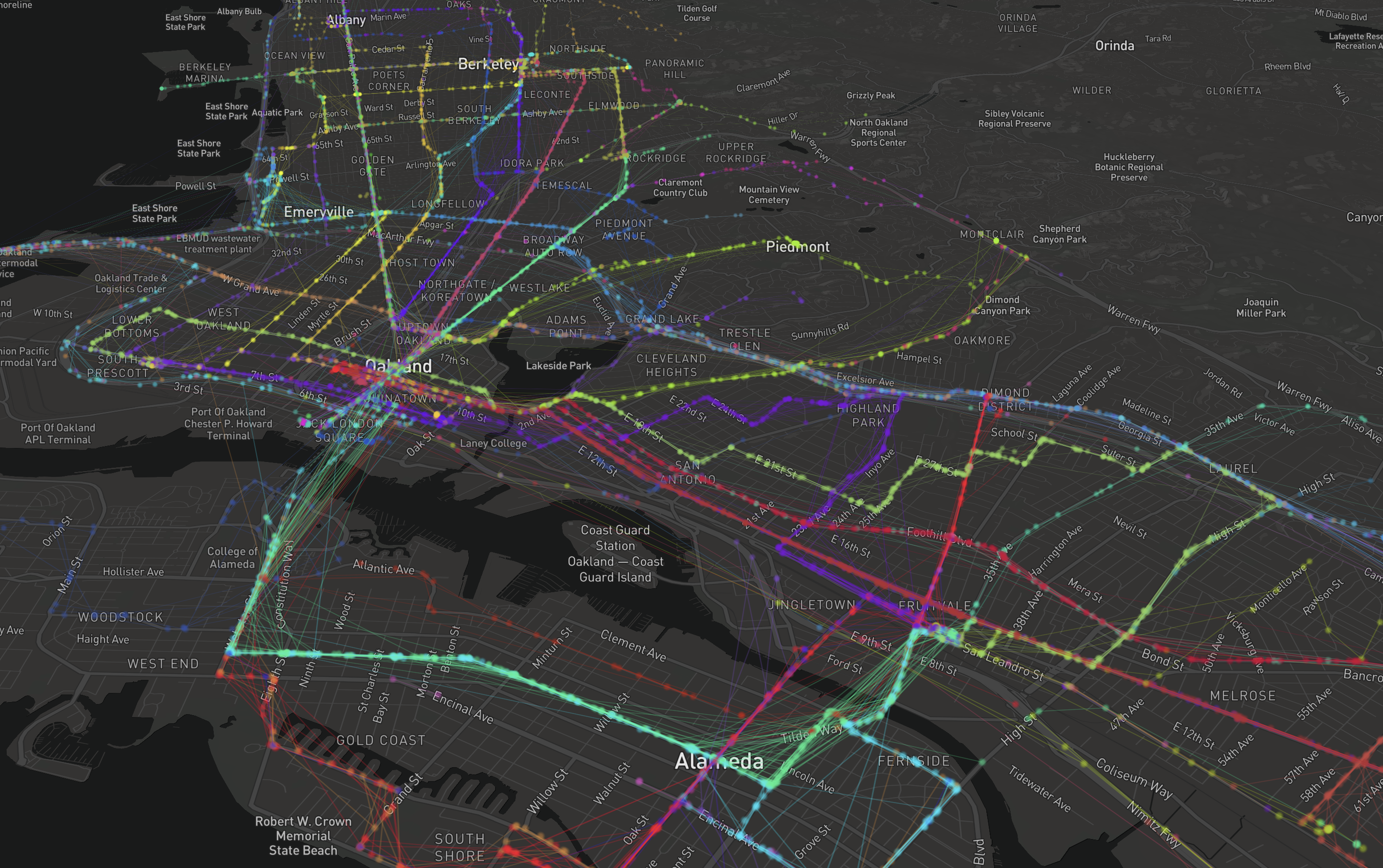
Above: Independent route traces of AC Transit buses from a recent Monday morning in the East Bay.

Introduction

I have found the AC Transit 18 bus to be an unreliable form of transit home, from Downtown Berkeley to MacArthur. I wanted to compare this bus line to the 6 line, which I “feel” performs better. The below logs how I went about gathering the data to perform a comparison.

Background

I have been logging all GTFS-RT vehicle location data for the active AC Transit fleet at 30-second intervals for a few weeks now. The set up is fairly simple and involves a micro virtual machine instance and plenty of cloud storage. For the purposes of this post, I’ll simply state that I have a dataset of all vehicle locations in the AC Transit network that are active, at 30-second intervals, for a few weeks’ time. Each dataset is held as a JSON representation of the GTFS-RT (real time) protobuf.

You can see what this looks like, visually, in the image at the top of this post.

Selecting the site

I want to geofence my analysis to the area that covers the route segment from downtown Berkeley to just south of 38th St. in Oakland, where both routes pass under the freeway.

I create a simple Polygon with which I will subset the routes by:

from shapely.geometry import Polygon

# We do not want to any of the route segments outside this area
boundary = Polygon([ [ -122.27937698364256, 37.865367675937094 ], [ -122.27491378784181, 37.86021777498129 ], [ -122.27439880371094, 37.849239153483246 ], [ -122.27045059204102, 37.83459844833992 ], [ -122.2719955444336, 37.82659905787503 ], [ -122.25740432739258, 37.82253123860035 ], [ -122.23920822143553, 37.85045908105493 ], [ -122.24281311035156, 37.86035330330106 ], [ -122.24959373474121, 37.86916210952103 ], [ -122.27937698364256, 37.865367675937094 ] ])

Similarly, I extract the LineStrings representing the 18 and 6 routes and hold them like so (in this case, because it was just two routes, I redrew by hand as the ones supplied as a Shapefile by AC Transit were a bit of a mess):

# Generate reference dicts
shapes = {
    '6': LineString([ [ -122.26845502853392, 37.87216025143104 ], [ -122.26830482482909, 37.87082211277181 ], [ -122.26815462112427, 37.8704833396357 ], [ -122.26800441741943, 37.87000905462816 ], [ -122.26802587509157, 37.86916210952103 ], [ -122.26778984069824, 37.86765452314282 ], [ -122.267746925354, 37.86673979277693 ], [ -122.26731777191162, 37.86673979277693 ], [ -122.2651720046997, 37.86701082518027 ], [ -122.25897073745728, 37.867823916408895 ], [ -122.25852012634277, 37.86529991641881 ], [ -122.25849866867065, 37.86474089801567 ], [ -122.25892782211304, 37.86199656434886 ], [ -122.2598934173584, 37.85513528309431 ], [ -122.2603440284729, 37.852000905081574 ], [ -122.26088047027586, 37.84810392497392 ], [ -122.26107358932495, 37.84652813106081 ], [ -122.26133108139037, 37.84476591303736 ], [ -122.26167440414429, 37.84224112344709 ], [ -122.26201772689818, 37.839902650620914 ], [ -122.26229667663573, 37.837784404718995 ], [ -122.26248979568481, 37.8367167857294 ], [ -122.26354122161864, 37.8327003663711 ], [ -122.26607322692871, 37.82337871943924 ] ]),
    '18': LineString([ [ -122.26916313171387, 37.87841022277056 ], [ -122.26844429969788, 37.87217718973932 ], [ -122.26821899414061, 37.87066119572638 ], [ -122.26804733276367, 37.87023772813792 ], [ -122.2679829597473, 37.86995823819627 ], [ -122.26803660392761, 37.86932302984053 ], [ -122.26799368858337, 37.8686793464538 ], [ -122.267746925354, 37.86652804801818 ], [ -122.26726412773132, 37.862335376503815 ], [ -122.26710319519043, 37.8610817637503 ], [ -122.26717829704286, 37.86002295258498 ], [ -122.26720511913298, 37.85979001208735 ], [ -122.2671729326248, 37.85953589434124 ], [ -122.26703882217407, 37.859298716987745 ], [ -122.26700663566588, 37.85912930412515 ], [ -122.26691544055939, 37.85860835713299 ], [ -122.26685106754302, 37.85779939962793 ], [ -122.26666331291199, 37.85634664213515 ], [ -122.26649165153502, 37.85510986975439 ], [ -122.26629316806795, 37.853457983868175 ], [ -122.26613223552705, 37.85239482747752 ], [ -122.2659659385681, 37.85112833830147 ], [ -122.26582109928131, 37.84995925206008 ], [ -122.26563334465025, 37.84870542882371 ], [ -122.26543486118315, 37.84722284005461 ], [ -122.26533830165863, 37.846464590277364 ], [ -122.2651720046997, 37.84519799923797 ], [ -122.26508080959319, 37.84446938182696 ], [ -122.26486086845398, 37.843029070416236 ], [ -122.26463556289671, 37.8410380053835 ], [ -122.26455509662627, 37.840487275778315 ], [ -122.26525783538818, 37.84036865655589 ], [ -122.26746797561646, 37.84009752618826 ], [ -122.26955741643907, 37.839813685516845 ], [ -122.26967275142668, 37.83980521264418 ], [ -122.26975589990617, 37.83979038511469 ], [ -122.26980149745941, 37.83978403045829 ], [ -122.2698175907135, 37.83975437538782 ], [ -122.26975321769713, 37.83950442503443 ], [ -122.2696003317833, 37.838915555599264 ], [ -122.26949572563171, 37.838667720654364 ], [ -122.26926773786543, 37.83810638201648 ], [ -122.26898610591887, 37.83761282413776 ], [ -122.2685891389847, 37.8370853702222 ], [ -122.2681814432144, 37.836646881566075 ], [ -122.2679078578949, 37.836343962759656 ], [ -122.26771473884583, 37.83607493592362 ], [ -122.26751357316971, 37.83588640472154 ], [ -122.26734459400177, 37.83568304468251 ], [ -122.26727217435837, 37.83557077275413 ], [ -122.26717025041579, 37.835280559619235 ], [ -122.26713806390764, 37.834986108629465 ], [ -122.26725608110426, 37.83444380732816 ], [ -122.26843357086182, 37.829870099886904 ], [ -122.2697639465332, 37.82442958216432 ] ])
}

Parsing the data

Now that I have my reference object, I can begin looking at my trace data. Again, these are held as JSONs on a Google Cloud bucket and I’ve pulled down values from the week of May 20th, locally, to play with.

target_files = [os.path.join(target_dir, f) for f in os.listdir(target_dir) if f.endswith('.json')]
print('Evaluating {} files'.format(len(target_files)))

This prints “Evaluating 11437 files.” That corresponds to roughly 4 days of trace data (Monday through Thursday). This is the data we will be working with.

Loading each line

First we need to parse out just the 18 and 6 line data, and hold them separately:

# Initialize tracking dict
compiled_traces = {}
for r in want_routes:
    compiled_traces[r] = []

for target_file in target_files:
    traces = None
    with open(target_file) as f:
        traces = json.loads(f.read())

    # Sometimes you don't get GTFSRT data...
    if 'entity' not in traces:
        continue

    for e in traces['entity']:
        veh = e['vehicle']
        trip = veh['trip']
        rid = str(trip['routeId'])
        rid = rid.split('-')[0]
        if rid in want_routes:
            compiled_traces[rid].append(veh)

Note that want_routes is just a list of the names we are interested in, which is [‘6’, ’18’].

Separating by direction

Now, I actually want just the southbound routes. So, a bit more manual parsing here, but I first pull out all trip ids that are in our subset list:

all_trip_ids = []

for r in want_routes:
    rows = []
    for ea in compiled_traces[r]:
        tid = ea['trip']['tripId']
        all_trip_ids.append(int(tid))

Then, I want to look at the GTFS for this season (their spring 2018 release), and just get the head-signs for the directions that we care about:

tdf = pd.read_csv('act_explore/gtfs/trips.txt')
target_trip_ids = [s for s in set(all_trip_ids) if s in tdf.trip_id.unique()]
sub = tdf[tdf.trip_id.isin(all_trip_ids)]

# We list the head signs in the other direction that
# we _do not_ want in our results
mask = sub.trip_headsign.isin(['ALBANY', 'BERKELEY BART'])
keep_trip_ids = sub[~mask].trip_id.unique()

Now that I have a list of the trips we care about, I can subset our original list and just get back the traces for the southbound segments. For these segments, I can format them in a way that is conveniently converted into a pandas DataFrame:

from shapely.geometry import box, Point

def check_if_in_bounds(lat, lon, bounds):
    p = Point(float(lon), float(lat))
    return p.intersects(bounds)

compiled_traces_dfs = {}

for r in want_routes:
    line = shapes[r]
    rows = []
    for ea in compiled_traces[r]:
        tid = ea['trip']['tripId']
        
        # We only want southbound trips
        if int(tid) not in keep_trip_ids:
            continue
        
        lat = ea['position']['latitude']
        lon = ea['position']['longitude']
        if not check_if_in_bounds(lat, lon, boundary):
            continue
            
        # Otherwise, we can interpolate the point onto the route
        p = line.interpolate(line.project(Point(lon, lat)))
        portion = line.difference(box(-122.355881,37.632226,-122.111874,p.y))

        formatted = {
            'portion': round(portion.length/line.length, 2),
            'bearing': float(ea['position']['bearing']),
            'timestamp': int(ea['timestamp']),
            'trip_id': tid,
            'veh_id': ea['vehicle']['id']}
        rows.append(formatted)
    compiled_traces_dfs[r] = pd.DataFrame(rows)

Note that I use point interpolation against the route line from earlier:

p = line.interpolate(line.project(Point(lon, lat)))

This allows me to ensure I am always comparing the same line (“apples to apples”), which allows me to safely calculate the portion of the route that has been covered by that time stamp.

portion = line.difference(box(-122.355881,37.632226,-122.111874,p.y))

Also note that I use just a giant box to delete/crop out the bottom of the route. It just so happens that the routes are laid out in a way that lets me hack this together. A better solution would be to slightly buffer the interpolated point, perform an intersection, and drop all but the first segment of the route. But, this is just a quick analysis so, whatever!

Grouping and summary stats

Now I need to group the data by unique trip and vehicle. I need to do this so I can get the time difference since the route entered the top of the geofenced area and create a new “time since starting line” value (time delta). I want to do this because the routes start at different points so I could not reasonable compare them from their different time starts, otherwise.

def calc_time_delta(df):
    sorted_df = df.sort_values('timestamp')
    first_time = sorted_df['timestamp'].values[0]
    td = sorted_df['timestamp'] - int(first_time)
    sorted_df['timedelta'] = td
    deduped = sorted_df.drop_duplicates(subset=['timedelta'])
    deduped = deduped.reset_index()
    
    # Drop rows where it started at the end of the trip
    if deduped.portion.mean() > 0.7:
        return deduped.head(0)
    return deduped

def further_sort(df):
    return df.groupby('trip_id').apply(calc_time_delta)[['portion', 'timestamp', 'timedelta']]

Now, I can analyze one of the routes, like so:

df = compiled_traces_dfs['18']
parsed = df.groupby('veh_id').apply(further_sort)
parsed.to_csv('18_parsed.csv')

Performance results

I would like to compare the performance of the two routes in terms of their consistency. I do so with the following script:

import matplotlib.pyplot as plt
fig, ax = plt.subplots(facecolor='white')
max_res = parsed.groupby('veh_id')['timedelta'].max()
max_res_sub = max_res[max_res < (45 * 60)]
ax = pd.Series(max_res_sub / 60).hist(bins=10)
ax.set_xlim(10,30)
ax.set_ylim(0,10)
ax.set_title('18 bus segment run time distribution (std: {} min)'.format(round(np.std(max_res_sub / 60), 2)))

This allows me to see the spread of run times over the week, as well as the standard deviation. From these results, I can see that both the 18 and 6 bus perform roughly equivalent along their respective paths.

compare-plots

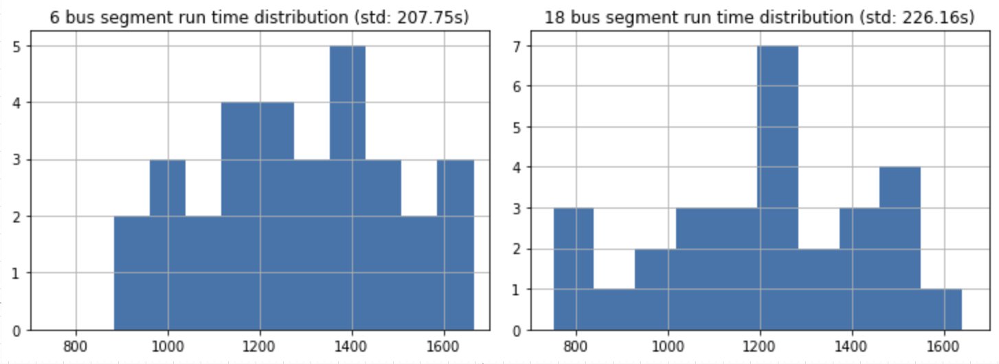
This is in contrast to what I perceived as more poor performance along the 18 line. I chalk this up to the flaws of human perception and personal experience. In aggregate, the data shows that the 18 appears to be comparable along its path to MacArthur as the 6 bus is.

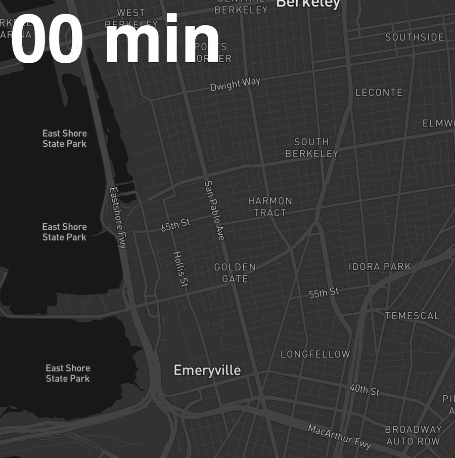
Let’s view this on a map

Let’s create the following visual, where width is a function of the percent of all buses along this segment that have passed through that segment by the time shown in the top right. (Basically, the 6 and the 18 are neck and neck.)

animated

First, we need to convert the line shape data for each route into a series of segmented lines. Doing so will allow us to attribute the portion of the trip that segment corresponds to with the number of buses out of all vehicles that have passed through that segment by a given time.

We can do this in a hacky way with the following:

from shapely.geometry import LineString, MultiPoint, MultiLineString
from shapely.ops import split

def process_coords(g):
    cleaned = [list(xy) for xy in g.coords.xy]
    return [[x, y] for x, y in zip(*cleaned)]

def convert_to_coords(name):
    line = shapes[name].simplify(0)
    n = 20
    s = 0.000000001
    splitter = MultiPoint([line.interpolate((i/n), normalized=True) for i in range(1, n)]).buffer(s)
    mls = MultiLineString(split(line, splitter))
    mls = [g for g in mls if g.length > s*2]
    return [process_coords(g) for g in mls]

Note that the second function trims out a small bit from each part of the route to break it into 20 discrete segments. Each segment is 1/20th of the total route. So, we will be thinking of the route in 5% chunks.

We can save the results as a list like so:

import json

coords_6 = convert_to_coords('6')
with open('coords_6.json', 'w') as outfile:
    json.dump(coords_6, outfile)

Using Mapbox GL JS to render this on a map

I’ll just breeze over this segment, as it’s a fairly conventional implementation of MB GL JS.

Suffice to say, we add the following layer source to the map:

map.addLayer({
    'id': `ref-${id}-lines`,
    'type': 'line',
    'source': {
        'type': 'geojson',
        'data': featureCollectionLines,
    },
    'paint': {
        'line-color': light_color,
        'line-opacity': 0.75,
        'line-width': ['get', 'weight'],
    }
});

Then, we create an incrementing interval-set function that will update each of the 20 segments as the time goes up. The component that resets the source layer’s reference data looks like this (super hacky, but just to provide a rough idea):

// Array incrementing by 0.05, where breaks variable
// is a list of values [0.05, 0.1, ... 0.95, 1]
var counts = breaks.map(function(brk) {
    var vehs = [];
    bustimes.forEach(function (bt) {
        if (!vehs.includes(bt.veh_id)) {
            vehs.push(bt.veh_id);
        }
    })

    var pass_vehs = []
    bustimes.filter(function (bustime) {
        return Number(bustime.timedelta) <= elapsed;
    }).filter(function (bustime) {
        return Number(bustime.portion) >= brk;
    }).forEach(function (ea) {
        if (!pass_vehs.includes(ea.veh_id)) {
            pass_vehs.push(ea.veh_id);
        }
    })
    return pass_vehs.length/vehs.length;
})

This resulting list is then multiplied by, say, 10, and each value reapplied to the relevant properties component in the GeoJSON feature collection. The resulting updated GeoJSON is reset against the Mapbox layer like so:

map.getSource(`ref-${id}-lines`).setData(featureCollectionLines);

Final thoughts

If you’ve got any other ideas for analysis of AC Transit bus performance data, feel free to hit me up and pass it along!

Corridor analysis with GTFS-RT trace data