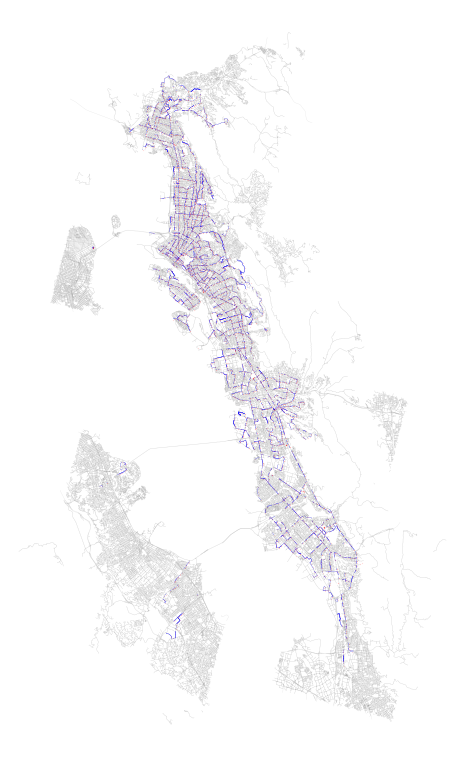
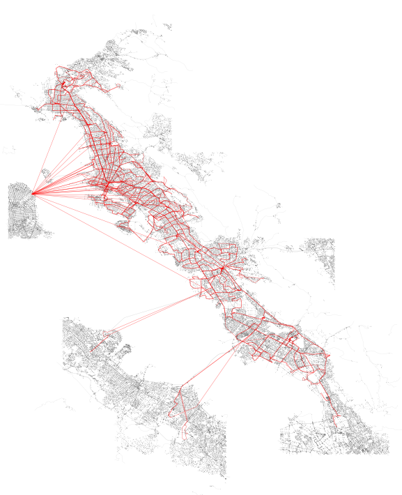
Above: SharedStreets (SS) segments tethered to transit stops in blue, analyzed transit stops from AC Transit in red, all OSM geometries associated with selected SS tiles in grey.
Introduction
The intent of this post is to document some initial exploration with the SharedStreets format in conjunction with GTFS data processed with Peartree. In this post, I use correlate Peartree data to SharedStreets (SS) and, via linearly-referenced system, am able to perform walk analyses from network stops (bus stops) in Peartree and map out transit + walk accessibility against SharedStreets segment metadata (which is from OpenStreetMap OSM). That said, once I have tethered the Peartree network graph stops to SS segments, I observe how I can interchange OSM data for other network datasets also associated with SS, and compare walk segment outputs easily through the SS medium.
Background
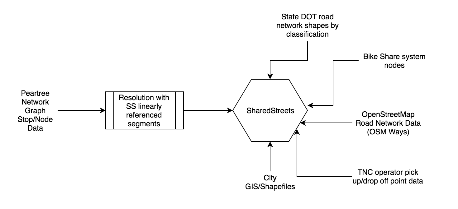
SharedStreets (SS) is an interesting platform. By creating a linearly referenced system approximating known paths around the world, it creates a medium through which disparate datasets - from city sidewalk data to OpenStreetMap road network data to state road network shape files - can “speak to one another.”
As a medium through which these datasets speak, one must only tether their data to SS. Once that has been accomplished, identifying likely comparable segments in other datasets is also possible.
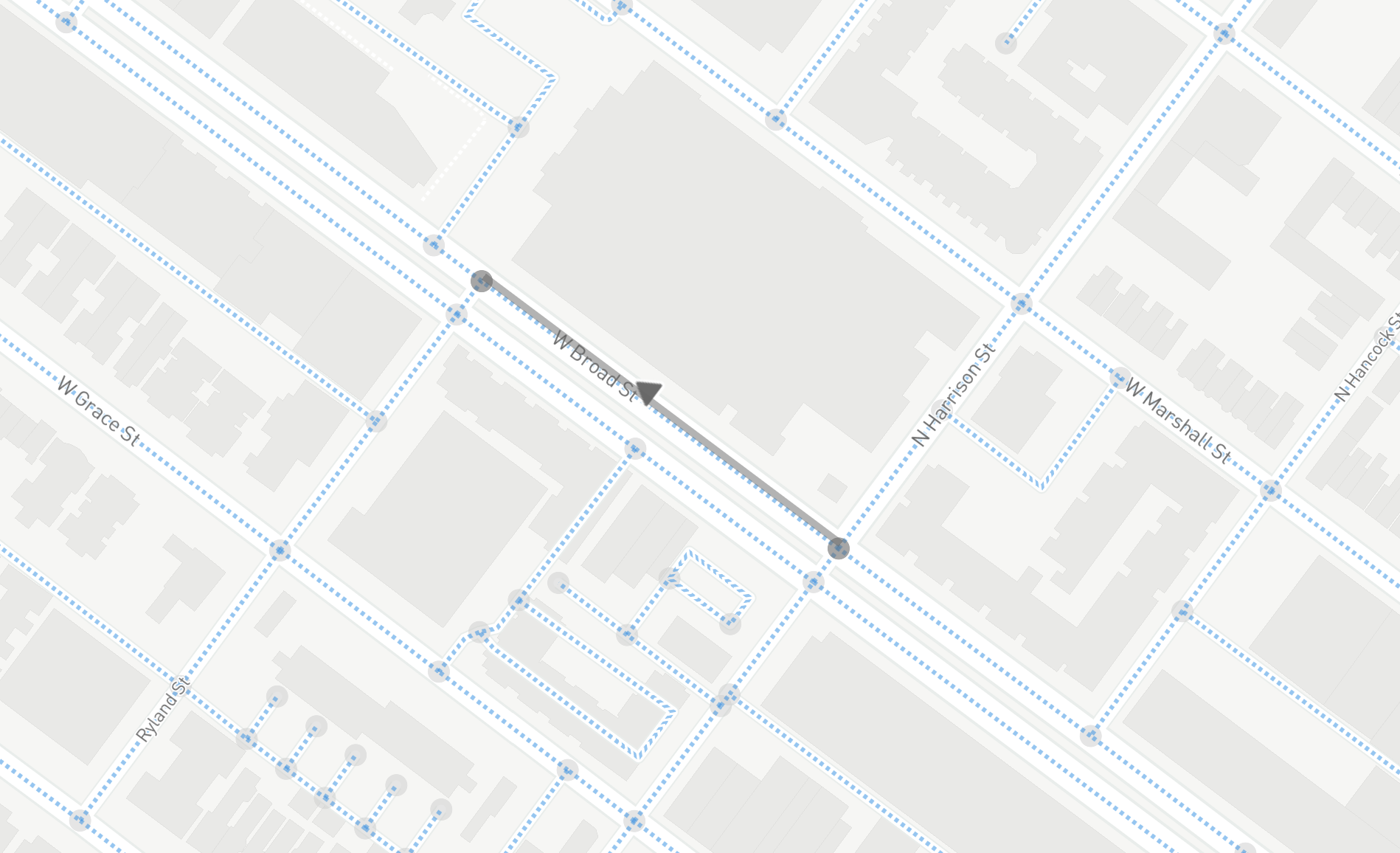
In the above image, taken from an exploratory interface available via SharedStreets, one can see the cleaned road segments shown on top of Mapbox map tiles (which render OpenStreetMap road segments, or “ways”).
Loading in transit network data
Let’s start with something I’ve likely blogged about more than a few times and load in some transit network data with Peartree.
There’s nothing unusual here, we will just load in the default busiest schedule data as a directed network graph:
import peartree as pt
path = 'act_explore/gtfs.zip'
feed = pt.get_representative_feed(path)
start = 7*60*60 # 7:00 AM
end = 10*60*60 # 10:00 AM
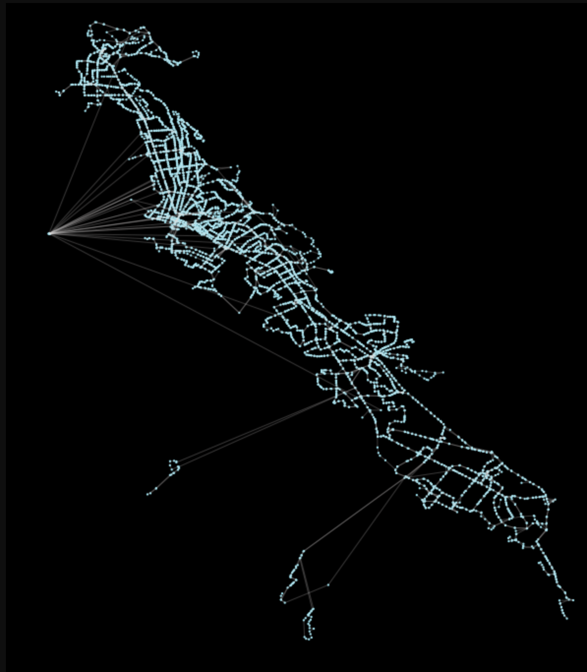
Gac = pt.load_feed_as_graph(feed, start, end)Plotting the results with the library’s built-in pt.generate_plot should generate the image shown prior, with the network in blue on a black background.
Identifying SharedStreets vector tiles
Right now, I will be querying for SharedStreets vector tiles for map zoom 12. This seems to be a sufficient size, particularly as the edges themselves do not hold geometric data and thus are fairly small to pull down. What’s nice about this is that edge network data and the geometries they represent have been decoupled. Thus, once we get our data into SS segment pairs, we will be “untethered” (theoretically) from geometric data. This should vastly improve all sorts of analyses.
In order to do this, we will need to roughly capture the nodes of the transit network touch. This is easy to extract from the network graph. From those nodes, we will buffer them roughly by 0.03 degrees which is about 2 miles in the Bay Area. This can be rough as we just need to make sure we hit the edges of all the tiles we will roughly need and if we pull in one or two extra, that is okay.
We can accomplish this with the following method
import sharedstreets.tile

def generate_geojson_of_coverage_area_streets(G, z=12):
    geojson_master = None
    for mt in _generate_tile_coordinates(G, z):
        tile = sharedstreets.tile.get_tile(z, mt.x, mt.y)
        geojson = sharedstreets.tile.make_geojson(tile)

        if geojson_master is None:
            geojson_master = geojson

        else:
            # Updates both the features and references keys
            for key in ['features', 'references']:
                fs = _filter_new_objects(geojson_master, geojson, key)
                geojson_master[key].extend(fs)
    return geojson_master
Which in turn relies on these 2 helper functions:
import mercantile
from shapely.geometry import Point

def _generate_tile_coordinates(G, z):
    mts = []
    for i, n in list(G.nodes(data=True)):
        # Now perform a buffer around the node points
        # to get a rough estimate of everything within
        # about 2 miles of the node
        p = Point(n['x'], n['y'])
        bp = p.buffer(0.03)  # 0.03 is about 2 miles
        bpe = bp.simplify(0.005).exterior
        for x, y in zip(*bpe.coords.xy):
            mt = mercantile.tile(x, y, z)
            mts.append(mt)

    # Dedupe results
    return set(mts)


def _filter_new_objects(master, new_gj, key):
    keep = []
    gm_ids = [f['id'] for f in master[key]]
    for f2 in new_gj[key]:
        if f2['id'] not in gm_ids:
            keep.append(f2)
    return keep
These two helper functions perform the buffer, use Mapbox’s mercantile library to get the conversion from web mercator coordinates to vector tile coordinates (quadrant-based x, y values).
From these methods, we can generate a JSON which represents the parsed protobuf vector tiles from SharedStreets, representing all tiles in related to the Peartree network graph:
# Generate a GeoJSON Feature Collection of the total coverage area
ssgj = generate_geojson_of_coverage_area_streets(G)
From these results, we can quickly plot the output to visually observe the network graph on top of the SharedStreets graph:
SharedStreets Python library
The SharedStreets Python library allows for easily interfacing with the SharedStreets API. It’s part of the SharedStreets organization on Github and its repo is here.
There are two components in a returned object:
- The references (the graph itself, with reference IDs for related components) as a list of references.
- The geometries, which are referenced by ID in the references list. The geometries are also held as a list of objects.
Combing the two is possible by first creating a lookup from the reference to the geometries, like so:
geometry_lookup = {}
for feature in ssgj['features']:
    i = feature['id']
    geometry_lookup[i] = feature

shaped_references = []
for r in ssgj['references']:
    feature = geometry_lookup[r['geometryId']]
    r['feature'] = feature

    # Also convert all distances to meter from centimeter
    for lr in r['locationReferences']:
        d = lr['distanceToNextRef']
        if d is not None:
            lr['distanceToNextRef'] = d/100.0

    shaped_references.append(r)
By doing this, we can improve the quality of the visualization of the network from straight edge connections, such as this detail:
To plots that look like this, with this level of detail:
Now, this is not important for the analysis of the network except for the fact that we can calculate the real length of the edge, instead of the straight line distance. This will make calculating walk times along edges more accurate. It will also help for the initial step of identifying which network node is assigned to which SharedStreets edge.
Note that in the prior plotted graph with the whole system, each edge was not “fully” rendered and thus the detail shown in the 2nd of the 2 plots above was absent.
Next, we can iterate through both the nodes (via intersectionId) and the edges (via the same, but in paired form), to generate a GeoDataFrame:
from functools import partial
import geopandas as gpd
import pandas as pd
import pyproj
from shapely.geometry import Point
from shapely.ops import transform

project = partial(
    pyproj.transform,
    pyproj.Proj(init='epsg:4326'),  # source coordinate system
    pyproj.Proj(init='epsg:2163'))  # destination coordinate system

# Generate nodes based on intersectionId
nodes = []
for sr in shaped_references:
    for lr in sr['locationReferences']:
        p = Point(lr['point'])
        pp = transform(project, p)  # apply projection
        new_row = {
            'id': lr['intersectionId'],
            'geometry': p,
            'x_meter': round(pp.x),
            'y_meter': round(pp.y)
        }
        nodes.append(new_row)

# Then convert to a pandas DataFrame and drop duplicates
nodes_df = pd.DataFrame(nodes)
nodes_df = nodes_df.drop_duplicates(subset=['id'], keep='first')
nodes_gdf = gpd.GeoDataFrame(nodes_df, geometry=nodes_df.geometry)

# Create the edges dataframe
edges = []
for sr in shaped_references:
    # Only do for direct edges (which should be all)
    if len(sr['locationReferences']) == 2:
        lrs = sr['locationReferences']
        if lrs[0]['sequence'] == 0:
            first = 0
            last = 1
        else:
            first = 1
            last = 0

        lrs = sr['locationReferences']
        fr = lrs[first]['intersectionId']
        to = lrs[last]['intersectionId']
        d = lrs[first]['distanceToNextRef']
        edges.append({
            'id': sr['id'],
            'from': fr,
            'to': to,
            'length': d,
            'geometry': shape(sr['feature']['geometry'])
        })

    # This should not ever happen
    else:
        # Could actually use logger instead of a print statement
        print('Skipped an edge - not length 2')

edges_df = pd.DataFrame(edges)
edges_df = edges_df.drop_duplicates(subset=['id'], keep='first')
edges_gdf = gpd.GeoDataFrame(edges_df, geometry=edges_df.geometry)
Comment on edge classifications
For the purposes of this exploration, I simply accepted that I was going to use all edges of the network. In reality, I would likely want to parse out walk networks, or perhaps only highways. Right now, that is not particularly easy to do with SharedStreets.
Reprojection
Since we will be performing a series of distance and buffer-related calculations, we should convert the GeoDataFrames into a meter-based projection. This will help ensure we are more accurate in our geometric operations.
Above: The results of the reproduction of the edge GeoDataFrame.
The code to do this is quite simple:
# Reproject project in equal area meter
project = partial(
    pyproj.transform,
    pyproj.Proj(init='epsg:4326'),  # source coordinate system
    pyproj.Proj(init='epsg:2163'))  # destination coordinate system

edges_gdf_reproj = edges_gdf.copy()
edges_gdf_reproj['geometry'] = edges_gdf_reproj['geometry'].apply(lambda g: transform(project, g))
Pairing to SharedStreets
At this point, we have the SharedStreets network in a GeoDataFrame, which will make resolving the AC Transit peartrees graph network easier. Now, this is definitely a step that could be far more optimized, but since this is a casual weekend exploration, and performed within a single Jupyter notebook, no effort was made to optimize (or, specifically, parallelize) this step. As a result, runtime against all edges in the related network on all 5,050 graph nodes took about 1.5 hours. The script to find the nearest edge to each network node is fairly straightforward, simply iterating through all edges in a loop. I acknowledge that even simple optimizations such as the inclusion of a spatial index could have drastically sped this up. I include it here only so someone else might use it as a starting point for performing a similar task in the future:
import numpy as np

nodes_to_consider = []
for i, node in G.nodes(data=True):
    node_p = transform(project, Point(node['x'], node['y']))  # apply projection
    nodes_to_consider.append((i, node_p))

print('Eval {} nodes'.format(len(nodes_to_consider)))

def min_dist(point, gdf, max_d):
    # Get all possible road segments that are within 50 meters of the node
    gdf_sub = gdf[gdf.intersects(point.buffer(50))]
    gdf_sub = gdf_sub.reset_index(drop=True)

    # Calculate the shortest distance to all these subset segments
    dists = []
    for geom in gdf_sub.geometry:
        d = point.distance(geom)
        dists.append(d)

    # Bail early if nothing to compare with
    if len(dists) == 0:
        return None

    # Note: min_dist is in meters
    dists = np.array(dists)
    dm = dists.min()

    # Do not allow "too-far" distances
    if dm > max_d:
        return None

    # Otherwise return the smallest distance row
    row = gdf_sub.iloc[dists == dm].head(1).squeeze()
    distance_along = row.geometry.project(point)
    return {
        'row': row,
        'distance_along': distance_along,
        'percentage_along': distance_along/row.geometry.length}

assoc_segments = []
for i, node_p in nodes_to_consider:
    closest = min_dist(node_p, edges_gdf_reproj, 25)

    # Only if there is one found
    if closest is not None:
        g = closest['row'].geometry
        ss_id = closest['row']['id']
        fr_ss_id = closest['row']['from']
        to_ss_id = closest['row']['to']
        distance_along = closest['distance_along']
        percentage_along = closest['percentage_along']
    else:
        g = None
        ss_id = None
        fr_ss_id = None
        to_ss_id = None
        distance_along = None
        percentage_along = None
    assoc_segments.append({
        'id': i,
        'ssid_edge': ss_id,
        'ssid_from': fr_ss_id,
        'ssid_to': to_ss_id,
        'geometry': g,
        'distance_along': distance_along,
        'percentage_along': percentage_along})

assoc_segments_df = pd.DataFrame(assoc_segments)
assoc_segments_gdf = gpd.GeoDataFrame(assoc_segments_df, geometry=assoc_segments_df.geometry)
We can now view the results of this effort by plotting the edges that were paired (in blue) on top of the plot of all edges in the network. In addition, I have marked the stops themselves in red.
What can we do with the paired network data?
Once we have the paired network data, we can begin to contextualize the transit network stops. For example, we can create buckets and see how much of the East Bay (since AC Transit served Oakland) can be accessed in 5, 10, 15, and 20 minutes from each bus stop. This can help visualize the coverage of the East Bay that the network has - ignoring frequencies and the transit network itself. It is just amount of the walk network that the nodes are in close proximity to.
Using a default walk speed of 4.8 km/h, we can script this out using NetworX’s ego graph method to calculate what is accessible from each paired edge for each time bucket:
access_level_buckets = {}
for walkshed_time in DEFAULT_WALKSHED_MINUTES_BINS:
    accessible_edges = []
    analyzed_nodes = []
    for i, row in assoc_segments_gdf.iterrows():
        # First calculate walk time to either end of the edge
        distance_along = row['distance_along']
        percentage_along = row['percentage_along']

        # Note that all distances are in meters
        full_dist = distance_along / percentage_along
        remaining_dist = full_dist - distance_along

        time_first = ((distance_along / 1000) / WALK_SPEED_KMPH) * 60
        time_second = ((remaining_dist / 1000) / WALK_SPEED_KMPH) * 60

        # We need to iterate through two combinations - one is where the
        # agent walks to the start of the edge, and other to the end of the edge
        for center_node, time_radius in zip([row['ssid_from'], row['ssid_to']],
                                            [time_first, time_second]):

            # First make sure we have not already analyzed this intersection
            # already, to prevent repeating work
            if center_node in analyzed_nodes:
                continue
            else:
                analyzed_nodes.append(center_node)

            if not center_node:
                # print('Bailing becaue bad data: center '
                #       'node: {} and time: {}'.format(center_node, time_radius))
                continue

            # Calculate the amount of time left for the radius
            time_remaining = walkshed_time - time_radius

            # Bail if there is a miniscule amount of time left
            if time_remaining < 0.1:
                continue

            # Calculate all accessible edges of the graph from this given point
            subgraph = nx.ego_graph(G, center_node, radius=time_remaining, distance='cost')
            for fr, to, edge in list(subgraph.edges(data=True)):
                accessible_edges.append(edge['edge_id'])

    access_level_buckets[walkshed_time] = accessible_edges
Again, this is something that would be far more performant outside of NetworkX, but my intent is to just show this as a demonstration of potential - not something that would be used outside of a one-off.
With these results we can plot the output, with darker areas being closer to node points and those that are lighter being farther away. I found the results rather “pretty:”
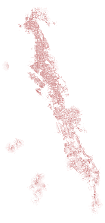
To plot this, I wrote the following:
# Just a set of reds, from dark to light
red_colors = ['#910707', '#d84949', '#f48484', '#fcbfbf']
# Hold onto the axis state between plots
ax = None
# Note: Reversing order of both so that lightest is drawn first, others
# are then stacked on top (as they get darker)
for accessible_edges_key, red in zip(reversed(DEFAULT_WALKSHED_MINUTES_BINS),
reversed(red_colors)):
# Get the keys we want to plot for this "level"
accessible_edges = access_level_buckets[accessible_edges_key]
sub = edges_gdf_reproj[edges_gdf_reproj['id'].isin(accessible_edges)]
# Plot parameters
a = 0.15
lw = 0.25
if ax is not None:
sub.plot(ax=ax, linewidth=lw, alpha=a, color=red)
else:
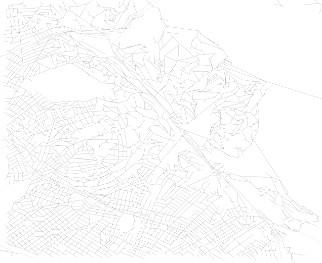
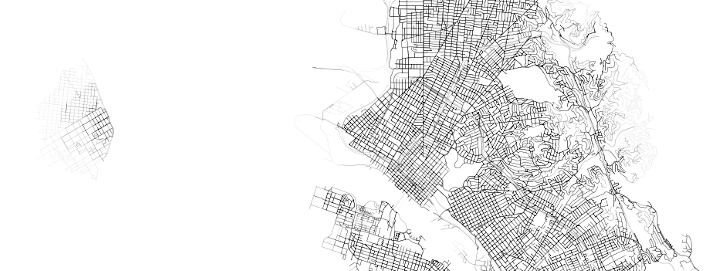
ax = sub.plot(figsize=(14,14), linewidth=lw, alpha=a, color=red)Looking in more detail (I plotted in black this time), we can explore certain parts of the city and see how transit + walk service exhibits itself.
For example, downtown Oakland is well serviced, and, to the west, downtown San Francisco is similarly well captured:
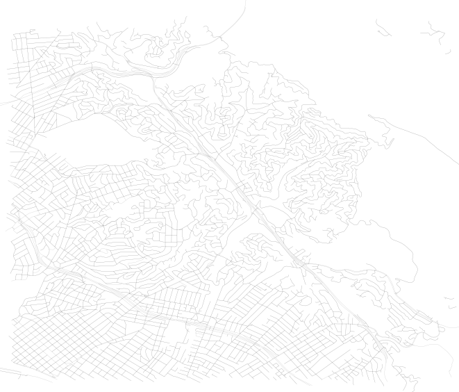
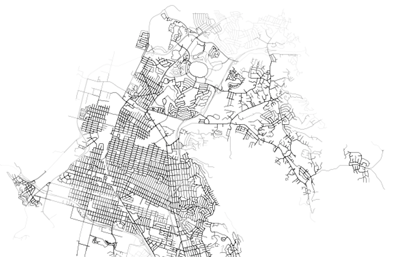
Looking north, we can see the core of Richmond is well serviced, but the suburban developments up the hill, as well as the areas around the large shopping mall, all have poorer levels of accessibility (20+ minutes to the nearest bus stop - any bus stop - is pretty bad).
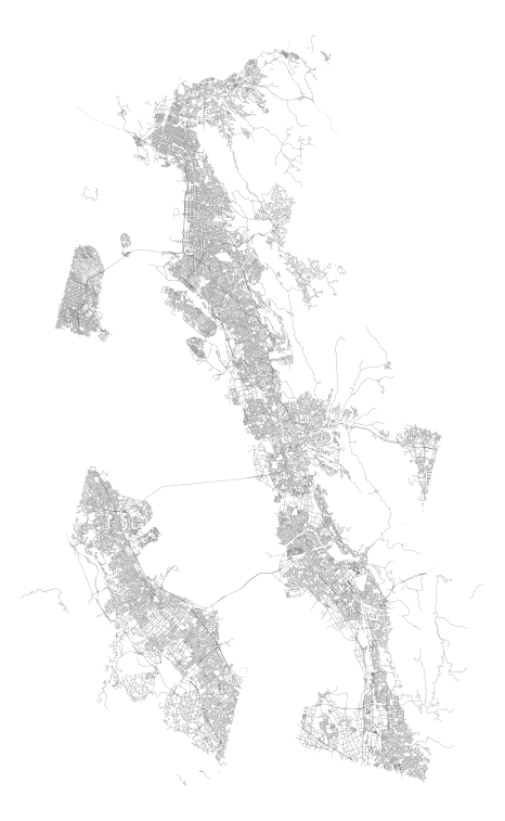
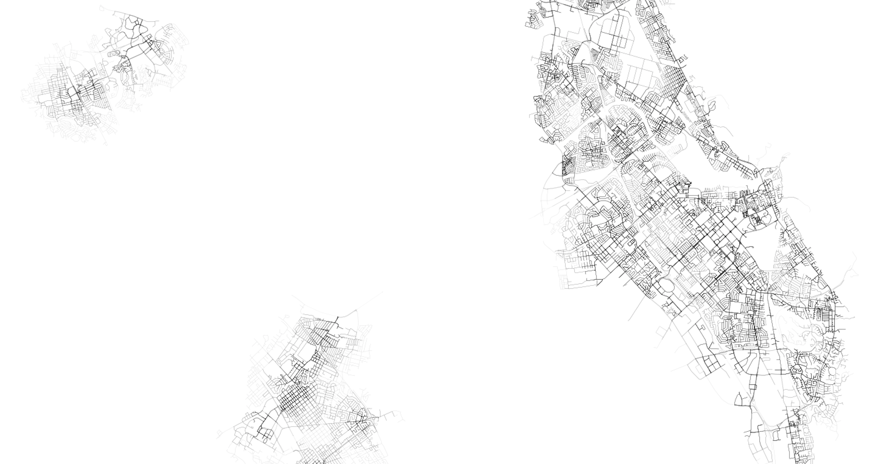
Finally, down south, we can see connections across the Bay to the peninsula. We can also see how suburban development and large swaths of freeway create greater inconsistency in transit coverage, with a tendency for “pockets” of access to transit nodes, surrounded by lower access areas that tend to be limited by the network components primarily designed to service vehicles.
Appending the transit network edges to the SharedStreets network
Now that we can neatly calculate walk shed from each edge that the transit network serves, we can also go ahead and add in the transit network itself. Below is a large blob of code but all it does is create a list of new edges to add that connect the network to the point on the edge in between the SS intersections and then also creates walk networks from that point to each of the intersections on the SS network (in both directions).
WALK_SPEED_KMPH = 4.8

# Making a new graph to work with, that
# includes the transit edges, too
G_mod = G.copy()

# Instantiate a list of new edges to add
edges_to_add = []
int_ids_to_add = []

# First, add in the edges from the transit graph
for fr, to, edge in Gac.edges(data=True):
    fr2 = fr.replace('1S53R', '6XK1T')
    to2 = to.replace('1S53R', '6XK1T')

    int_ids_to_add.append(fr2)
    int_ids_to_add.append(to2)

    edges_to_add.append({
        'from': fr2,
        'to': to2,
        'length': edge['length'],
        'edge_id': None,
        'cost': WALK_SPEED_KMPH * (edge['length'] / 1000)
    })

# Also need all edges from the graph to the walk network
# intersections, too (assuming all edges are walkable)
sub_asg = assoc_segments_gdf[~assoc_segments_gdf.geometry.isnull()]
for i, row in sub_asg.iterrows():
    # First calculate walk time to either end of the edge
    distance_along = row['distance_along']
    percentage_along = row['percentage_along']

    # Note that all distances are in meters
    full_dist = distance_along / percentage_along
    remaining_dist = full_dist - distance_along

    time_first = ((distance_along / 1000) / WALK_SPEED_KMPH) * 60
    time_second = ((remaining_dist / 1000) / WALK_SPEED_KMPH) * 60

    # We need to iterate through two combinations - one is where the
    # agent walks to the start of the edge, and other to the end of the edge
    for edge_node, dist, time_cost in zip([row['ssid_from'], row['ssid_to']],
                                          [distance_along, remaining_dist],
                                          [time_first, time_second]):

        # Make sure to do both directions for each
        edges_to_add.append({
            'from': row['id'],
            'to': edge_node,
            'length': dist,
            'edge_id': None,
            'cost': time_cost
        })

        edges_to_add.append({
            'from': edge_node,
            'to': row['id'],
            'length': dist,
            'edge_id': None,
            'cost': time_cost
        })
Now that the list has been created, we can iterate through it and add each new component to the copied network graph (which will now house both the SS network and the transit edges).
# Add new edges to the existing network graph
G_mod.add_nodes_from(list(set(int_ids_to_add)))

for new_edge in edges_to_add:
    if new_edge['length'] >= 0 and new_edge['cost'] >= 0:
        G_mod.add_edge(new_edge['from'],
                       new_edge['to'],
                       length=new_edge['length'],
                       edge_id=new_edge['edge_id'],
                       cost=new_edge['cost'])
    else:
        print('Skipping due to negative edge cost')
        print(new_edge['length'], new_edge['cost'])
Analyzing full network with transit
Now that we have a new graph object that contains both the “walk” SharedStreets network (again, remember I am assuming all components are ok for walking, but could have done some parsing back at the beginning to trim out highway segments or other car-only segments), we can generate accurate isochrones with the SS segments.
Let’s find the nearest node in to the 12th St/City Center Bart station in downtown Oakland:
dt_oak = Point(-122.271676, 37.803574)
project = partial(
    pyproj.transform,
    pyproj.Proj(init='epsg:4326'),
    pyproj.Proj(init='epsg:2163'))
dt_oak = transform(project, dt_oak)

# Calculate the distance to all nearby edges
egr_sub = edges_gdf_reproj[edges_gdf_reproj.geometry.intersects(dt_oak.buffer(100))]
# Calculate the shortest distance to all these subset segments
dists = []
for geom in egr_sub.geometry:
    d = dt_oak.distance(geom)
    dists.append(d)
dists = np.array(dists)

# Keep the nearest one
nearest = egr_sub[dists == dists.min()].head(1).squeeze()

# And return one of the paired intersectionIds
dt_oak_center = nearest['from']
We can now perform an ego graph to determine what part of the two networks is accessible in a given amount of time (let’s say 20 minutes) on the walk network or the modified network with transit (G would be swapped out):
accessible_edges_walk = []
subgraph = nx.ego_graph(G, dt_oak_center, radius=MAX_TIME_DEFAULT, distance='cost')
for fr, to, edge in list(subgraph.edges(data=True)):
    eid = edge['edge_id']
    accessible_edges_walk.append(eid)
First, we have results for 20 minutes, where walk is in green and walk plus transit is in purple:
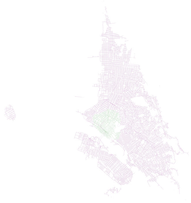
First, we have results for 40 minutes, where walk is in green and walk plus transit is in purple:
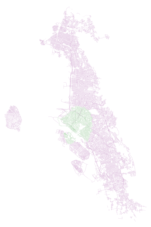
In both of these examples, we can see how AC Transit actually provides pretty decent coverage of the overall network. In spite of what I imagine would be a hard task (getting good coverage along the width of the East Bay instead of the length, where the longer main corridors of bus and Bart are), there appears to be good accessibility and high coverage (on weekdays, during peak hour, that is).
Script to generate those plots is like so:
transit_out_walk = list(set(accessible_edges_transit) - set(accessible_edges_walk))
sub = edges_gdf_reproj[edges_gdf_reproj['id'].isin(transit_out_walk)]
ax = sub.plot(figsize=(14,14), linewidth=0.25, alpha=0.25, color='purple')

sub = edges_gdf_reproj[edges_gdf_reproj['id'].isin(accessible_edges_walk)]
sub.plot(ax=ax, linewidth=0.25, alpha=0.25, color='green')
Conclusion
Shared streets is exciting because of its potential to be a “one and done” solution. That is, once I pair my network to SharedStreets and save that lookup table, I can potentially circumvent any future expensive geometric operations (so long as that other dataset has also been paired with SharedStreets). This helps create a “Rosetta Stone” of sorts where all metadata about segments can be stored and shared amongst disparate geospatial datasets.
Notes
Adding a thank you to Disqus user Pablo who noticed that time in minutes was being calculated incorrectly in the code snippets. An edit was made to address that on April 23, 2019.