Introduction
There’s no immediate way to export a GeoDataFrame to an SVG through, say, a Geopandas API method. That said, shapely object have a .svg() method that opens up the possibility for a GDF to SVG method to be easily developed. This post demonstrates a quick and dirty way of accomplishing this. It uses the data-* tag available on SVG elements to add each row value other than the geometry to each grouped row element.
Structure
The GDF to SVG method will group each row in a single group <g> tag. This allows that group tag (<g>) to hold all items from that row that are not the geometry value in data- tag form. A given row may have many polygons associated with it (held in a MultiPolygon). This allows the each polygon in that MultiPolygon to be nested within the group and the data attributes to be associated with those geometries only once. This is sufficient for portability and, for example, loading the associated data into a vector graphics tool like Adobe Illustrator, should that be desired (say you wanted to make a styled graphic of a GDF).
Example
For this exercise, I will use the zoning dataset from San Rafael, available here. This is a simple, typical Shapefile dataset that can be downloaded and loaded into Geopandas easily.
We can load it in pretty easily, and plot it:
%matplotlib inline
import geopandas as gpd

# Read in and reproject to equal area
gdf = gpd.read_file('san_rafael')
gdf.crs = {'init': 'epsg:4326'}
gdf = gdf.to_crs(epsg=2163)

# Plot the results to examine the dataset
plot_params = {
    'cmap': 'viridis',
    'figsize': (8,8)}
ax = gdf.plot(column='zoning', **plot_params)
ax.axis('off')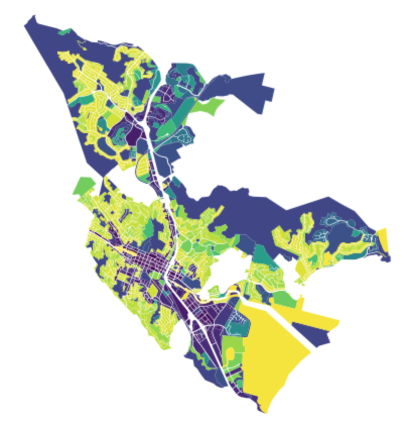
This will result in the above graphic.
Adjusting the coordinates
Now that we have the Shapefile converted to a GeoDataFrame, we need to adjust the coordinates so that they are “pushed” relative to a 0,0 coordinate position that represents the minimum x and y value from the coordinates of the GDF.
The below script does this. It finds the minimum x and y value and then, for each polygon (of each MultiPolygon) of each row, it shifts the x and y coordinates down so that the minimum of each axis then equals 0.
import numpy as np
from shapely.geometry import MultiPolygon, Polygon

min_x = None
min_y = None
extracted_xys = []
for row_geom in gdf.geometry:
    # Ensure same iterable pattern no matter what
    if isinstance(row_geom, Polygon):
        row_geom = [row_geom]

    all_geoms_in_row = []
    for g in row_geom:
        xys = g.exterior.coords.xy

        # Keep track of min values
        xs = np.array(xys[0])
        curr_min_x = xs.min()
        if min_x is None or min_x > curr_min_x:
            min_x = curr_min_x

        ys = np.array(xys[1])
        curr_min_y = ys.min()
        if min_y is None or min_y > curr_min_y:
            min_y = curr_min_y

        # Add to the row tally
        all_geoms_in_row.append(xys)

    # Add the row to the geodataframe tally
    extracted_xys.append(all_geoms_in_row)

shifted_geoms = []
for geom_group in extracted_xys:
    new_geom_group = []
    for xys in geom_group:
        adj_xs = np.array(xys[0]) - min_x
        adj_ys = np.array(xys[1]) - min_y
        new_geom_group.append(Polygon(zip(adj_xs, adj_ys)).simplify(10))
    shifted_geoms.append(MultiPolygon(new_geom_group))
We can check this result by plotting it again, this time with coordinates.
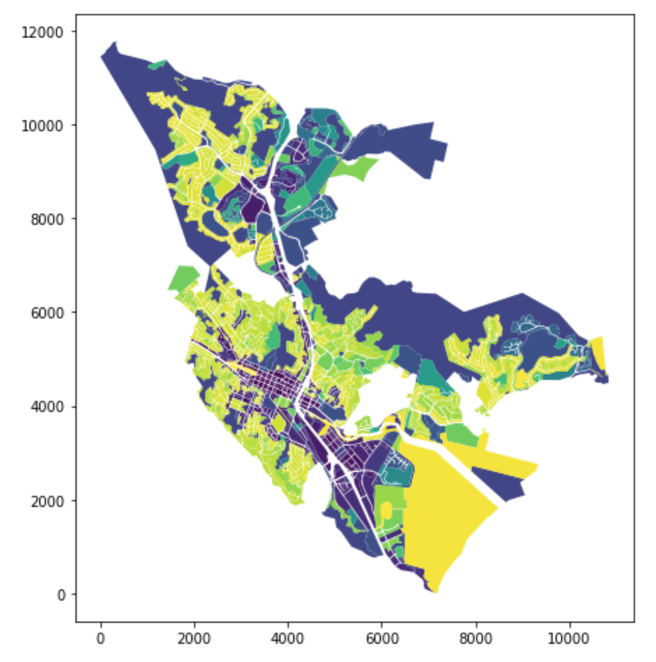
As we can see from the above result, the values are now relative to a 0,0 bottom left starting point.
Converting to an SVG string
At this point, we can just take a string representation of an SVG and replace the body of the SVG with the data pulled out from the rows in the GDF. We can first format each row using the below method.
def process_to_svg_group(row):
    orig_svg = row.geometry.svg()
    rd = row.to_dict()
    del rd['geometry']

    to_add = []
    for key, val in rd.items():
        to_add.append('data-{}="{}"'.format(key, val))

    return '<g {} >'.format(' '.join(to_add)) + orig_svg[3:]

processed_rows = []
for i, row in gdf.iterrows():
    p = process_to_svg_group(row)
    processed_rows.append(p)
In this method, we use the Shapely SVG method to get a string of the SVG, then we add the other row values in the top level <g> tag. Note that the returned SVG is defaulted to a green color if it is valid in Shapely and a red color if it is not. We can parse the returned string if we want to and change the color to whatever we want. For example, we could extract the viridis color scheme for the Geopandas plot and use that color result to apply the same colors to the geometries contained in each row and pulled out, here. I won’t go through the hassle in this post, but it is about as simple as adding in the data tags.
Speaking of data tages, we can insert those processed rows of the GDF into an SVG element, along with a bunch of standard default SVG tags. I also am going to set the width and height to a 100% so that the SVG will just scale to its parent div.
import textwrap

props = {
    'version': '1.1',
    'baseProfile': 'full',
    'width': '100%',
    'height': '100%',
    'viewBox': '{}'.format(','.join(map(str, gdf.total_bounds))),
    'xmlns': 'http://www.w3.org/2000/svg',
    'xmlns:ev': 'http://www.w3.org/2001/xml-events',
    'xmlns:xlink': 'http://www.w3.org/1999/xlink'
}
template = '{key:s}="{val:s}"'
attrs = ' '.join([template.format(key=key, val=props[key]) for key in props])

raw_svg_str = textwrap.dedent(r'''
    <?xml version="1.0" encoding="utf-8" ?>
    <svg {attrs:s}>
    {data:s}
    </svg>
''').format(attrs=attrs, data=''.join(processed_rows)).strip()
Finally, we can write the file to local storage, like so:
with open('test.svg', 'w') as f:
    f.write(raw_svg_str)
Performance
This isn’t a particularly optimized operation, but it looks like it runs decently. Running it in a loop 100x took about 99 seconds, so about 0.99 seconds per run. What I timed was the conversion to formatted string (so avoiding the IO part).
Given that performance on 1,801 row GeoDataFrame, we can assume that this should run decently quickly on larger data frames (particularly if a simplification step is included, as I did in this, to keep outputs at a reasonable level of detail.
Without simplification, the output file was 4.1 MB. With the 5 or 10 meter simplification (both were tried), it fall just below 1 MB.
Final result
To close out, here’s the SVG, embedded for download/to oogle at/etc.

Or as a Gist: