Calculating distance matrices is an inherently fraught endeavor as it’s cost increases exponentially with the number of points/geometries being considered (O(n^2)). Regardless, there are times when this is necessary.
In such cases, parallelization can be applied to reduce the overall runtime of the operation by breaking the compare list into chunks. In this post, I outline how Dask Delayed can be used to reduce runtime by a factor based on the number of cores made available to Dask Delayed.
For the purposes of the post, we will consider a typical operation: Given a set of centroids, we need to iterate through each coordinate pair (of which there can be N) and calculate the great circle distance between the two points. Wikipedia describes the great circle distance as the “shortest distance between two points on the surface of a sphere, measured along the surface of the sphere (as opposed to a straight line through the sphere’s interior).”
We can define the great circle vector operation with the following function. Please note that this method is adapted from the method of the same name from OSMnx. The repo for that project can be found here.
def great_circle_vec(
        lat1: float, lng1: float,
        lat2: np.array, lng2: np.array,
        earth_radius: int=6371009) -> float:
    phi1 = np.deg2rad(90 - lat1)
    phi2 = np.deg2rad(90 - lat2)
    theta1 = np.deg2rad(lng1)
    theta2 = np.deg2rad(lng2)

    arc = np.arccos(np.sin(phi1) * np.sin(phi2) \
          * np.cos(theta1 - theta2) \
          + np.cos(phi1) * np.cos(phi2))

    dist = arc * earth_radius

    # Return nothing; avoid memory issues
    # This issue will be discussed at the end of
    # the post, but is beside the point for
    # the example
    return None
In such an operation, we can create an immediate performance improvement by vectorizing each coordinate array as a Numpy array. Casting these float lists as Numpy arrays avoids risks of premature optimization by ensuring that the list of coordinates is being factored once per coordinate pair against the entire Numpy array.
Let’s look at what this looks like. First, let’s instantiate the x and y coordinates for 150,000 points with the following method. For the purposes of this example, we can just randomly create float values to evaluate the method performance with arbitrary data.
import numpy as np

N = 150_000
x = np.random.rand(N)
y = np.random.rand(N)
With the two vectorized arrays, we can now iterate through each coordinate pair and run the great circle vector method on the pair against the x, y vector arrays.
for x1, y1 in zip(x, y):
    great_circle_vec(x1, y1, x, y)
Unfortunately, this method will not scale: larger N values will create exponential performance regressions. So, for example, working with 10 centroids may take less than a second, but going to 100 centroids immediately jumps to about 1.7 seconds. Not good. Increase to a 1000 centroids and you are approaching 18 seconds, on average. As a result, it can quickly take minutes or hours to compute a pairwise distance matrix.
A solution to this is to run these computations in parallel. Each pairwise calculation against the full vector array can be run without impacting/needing the results of the other operations. As a result, we can leverage Dask’s Delayed package library to handle the parallelization of this operation.
We can set up the same operation using Delayed by simply arranging the method as a series of prepped methods wrapped in delayed operators. This allows Dask to orchestrate a map reduce operation, breaking up the for looped operation into a series of parallelized operations that are then collapsed back into a single result. In the below method, I wrap the for loop in a final len calculation. This is to visually confirm the length of the final output values (that is, that all values were run an N None values were returned, equivalent to the N coordinate pairs that were created.
result = delayed(len)([
    delayed(great_circle_vec)(x1, y1, x, y)
    for x1, y1 in list(zip(x, y))[:i]
])
Running on my 2013 MacBook Pro, with all 4 cores available, we can observe slight performance increases. These become more visible as N becomes higher, but, for example, N=1000 went down from almost 18 seconds to 10. At 10,000 centroids, performance went from about 145 seconds to 110 seconds.
What’s nice about the Dask Delayed set up, though, is that the operation can scale with the resources you provide it.
So, for example, I spun up a large VM instance on Google Cloud Platform. Specifically, I chose the 8 vCPUs 7.2 GB memory, n1-highcpu-8 machine type default. With 8 high performance CPUs, Dask Delayed was able to further fan out the mapreduce operation, dramatically reducing run time and, essentially, pushing the exponential cost curve further out “to the right.” 1000 centroids took 3.8 seconds (down from 18, and 10 seconds) and 10,000 centroids took 36 seconds (down from 145, and 110 seconds).
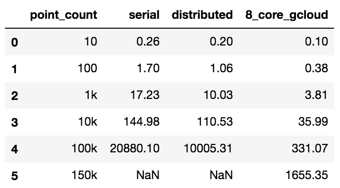
We can view the full performance table in the below:
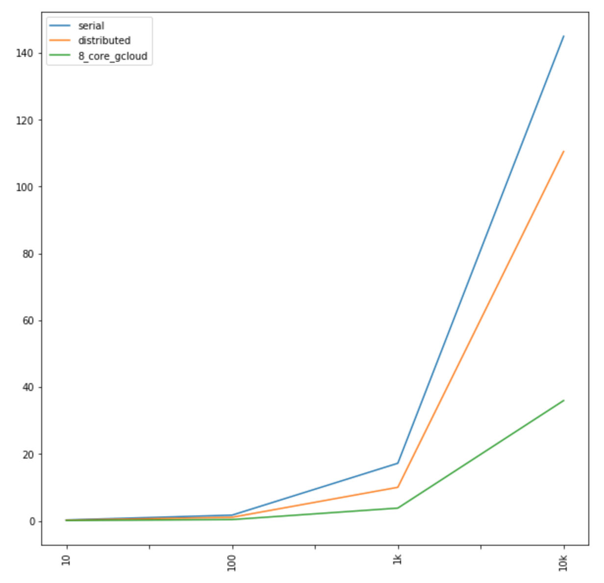
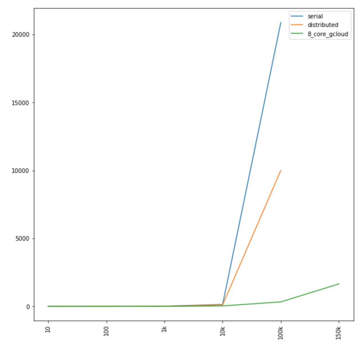
Similarly, we can see how much further we were able to push out the performance curve, by using better resourced VMs (x axis is count of coordinates N and y axis is time in seconds):
Zooming in on the x-axis, we can see where the divergence occurs, lower along the y-axis (x axis is count of coordinates N and y axis is time in seconds):