Introduction

The purpose of this post is to demonstrate a method for evaluating ideal grid size calculation from the perspective of performance when performing cell clustering. It is a follow up blog post to the one on performant spatial analysis via cell clustering from last week. Please read it first as this post builds off of that one.

In that previous post, I highlighted how you can quickly pin each geometry in a list of geometries to a cell representing all possible locations of geometries to certain degree of resolution in a large site comprised of 10s or 100s of thousands of geometries.

The purpose of the grinding operation is to cluster points to enable vectorized operations to be performed, leveraging the performance of numpy and avoiding expensive geospatial operations. In addition, such operations make interacting with large geospatial datasets possible in a notebook by summarizing them in a vectorized, aspatial format (that can still be plotted!).

The aim is specificity

Because we are aggregating geometries, we may desire to aggregate them as little as possible so as to preserve spatial accuracy as much as possible. As a result, we want to keep the size of the cell grid to be as small as possible.

There are a number of factors related to the performance, namely:

• The size of the target site (width, height)
• The size of the cell grid (e.g. in meters)
• The size of the evaluation window

The larger the evaluation window, the more cells that will need to be computed for each cells buffer cells. As a result, situations like a small cell size with a large buffer to be considered are recipes for creating non-performant situations.

The example method

For a given gridded dataframe, we want to take a “window” of n cells around a single cell and evaluate all those cells in that buffer area to process a contextually where descriptor attribute for a single gridded cell. The operation to do this is shown below:

def windows(x, window_radius):
    # Taken from the suggestion included in this numpy issue
    # https://github.com/numpy/numpy/issues/7753
    x = np.asarray(x)
    
    wshape = (window_radius, window_radius)

    try:
        nd = len(wshape)
    except TypeError:
        wshape = tuple(wshape for i in x.shape)
        nd = len(wshape)
    if nd != x.ndim:
        raise ValueError("wshape has length {0} instead of "
                         "x.ndim which is {1}".format(len(wshape), x.ndim)) 
    
    out_shape = tuple(xi-wi+1 for xi, wi in zip(x.shape, wshape)) + wshape
    if not all(i>0 for i in out_shape):
        raise ValueError("wshape is bigger than input array along at "
                         "least one dimension")

    out_strides = x.strides*2
    
    return np.lib.stride_tricks.as_strided(x, out_shape, out_strides)

We will apply that on every grid cell in the summary matrix of the original geometry collection.

Before doing so, though, we want to make sure to buffer the matrix so that we are able to run the window along the cells in the first row or the last row (or the first and last columns, too):

def create_windows_padding_frame(x, num_padding):
    x = np.asarray(x)
    
    row_margin = np.zeros((num_padding, x.shape[-1]), dtype=np.int32)
    # add top and bottom margin first
    x = np.concatenate((row_margin, x, row_margin), axis=0)
    
    col_margin = np.zeros((num_padding, x.shape[0]), dtype=np.int32)
    # add left and right margin then
    x = np.concatenate((col_margin.T, x, col_margin.T), axis=1)

    return x

The steps can then be combined like the below. In doing so, the operation takes in a given summary gridded matrix of cells and buffers it so that it can run the window over all the cells. Within each window, it sums all values from all cells to creating a floating sum paired with each cell.

# Create a gridded site of random values
gridded_site = np.random.rand(shape_y, shape_x)

# Create padding around the edge of the site so the floating buffer won't cause
# a reduced matrix shape size after application
padded_gridded_site = create_windows_padding_frame(gridded_site, window_cell_radius)

# Come up with the set of windowed areas
windowed = windows(padded_gridded_site, window_cell_diameter)

# Then apply an operation (in this case a simple sum) on each window
windowed_sums = np.array([np.sum(row, axis=1).sum(axis=1) for row in windowed])

Note that this summing operation is an arbitrary function for demonstration and benchmarking purposes. One could imagine a more involved operation that gets the mean, or evaluated the values distribution to identify local peaks, etc.

Creating a benchmarking operation

For the purposes of this post, we will work with a fairly large site and use that as our static component while evaluating dynamic cell size and window size variables. Thus the site will be 10 by 20 miles:

# Reference project size
x_miles = 40
y_miles = 20

We can now iterate over a series of differing cell sizes (in 25 meter increments), and window sizes (in integer values corresponding to the increasing cell sizes):

results = []
for cell_size_meter_i in range(10):
    cell_size_meters = 25 + cell_size_meter_i * 25

    for window_cell_radius in range(1,10):
        window_cell_diameter = 250 * wc_i
        window_cell_radius = math.ceil(window_cell_diameter/cell_size_meters)
        print('Cell size', cell_size_meters, ', Window count', window_cell_radius)

        start = time.time()

        # The radius is used to get the full square window
        # dimensions
        window_cell_diameter = (window_cell_radius * 2) + 1

        miles_to_meters = 1609.34

        x_adj = x_miles * miles_to_meters
        y_adj = y_miles * miles_to_meters

        shape_x = math.ceil(x_adj / cell_size_meters)
        shape_y = math.ceil(y_adj / cell_size_meters)

        cell_count = shape_x * shape_y

        # Create a gridded site of random values
        gridded_site = np.random.rand(shape_y, shape_x)

        # Create padding around the edge of the site so the floating buffer won't cause
        # a reduced matrix shape size after application
        padded_gridded_site = create_windows_padding_frame(gridded_site, window_cell_radius)

        # Come up with the set of windowed areas
        windowed = windows(padded_gridded_site, window_cell_diameter)

        # Then apply an operation (in this case a simple sum) on each window
        windowed_sums = np.array([get_normalized_row_vals(row) for row in windowed])

        end = time.time()

        results.append({
            'cell_size': cell_size_meters,
            'cells_window': window_cell_radius,
            'cells_radius': (window_cell_radius * cell_size_meters),
            'cell_count': cell_count,
            'runtime': round(end - start, 5),
        })

Visualizing the results

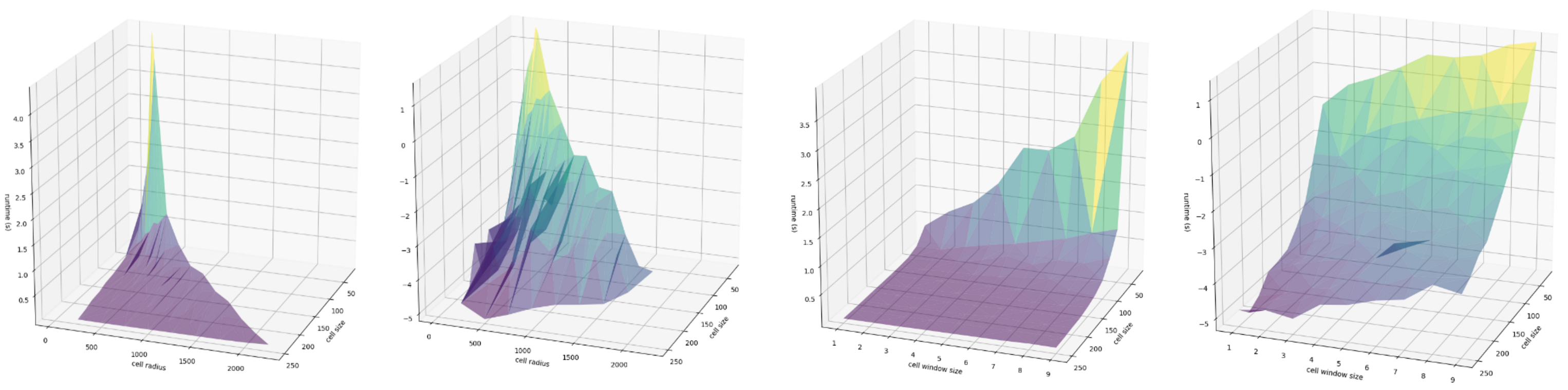
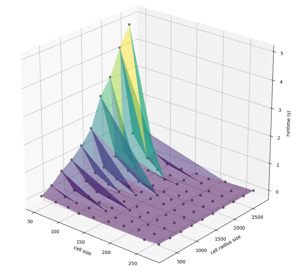
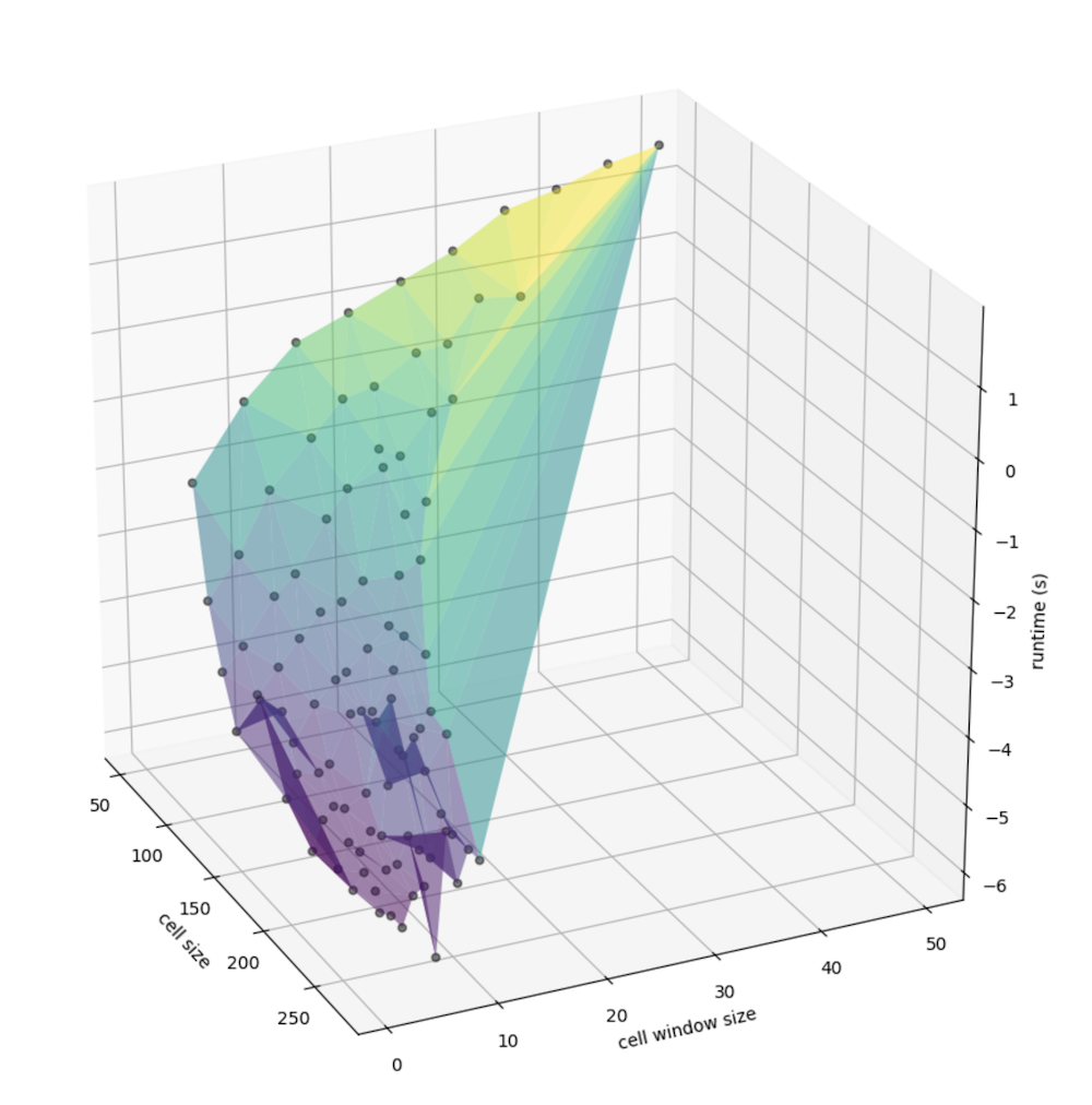
At this point, we can convert that information into a DataFrame for portability and plot amongst a number of factors. First, let’s explore the relationship between the computed cell radius (the window size multiplied by the cell resolution, in meters) the cell size (the width an height of a given singe cell, also in meters), and the runtime in seconds:

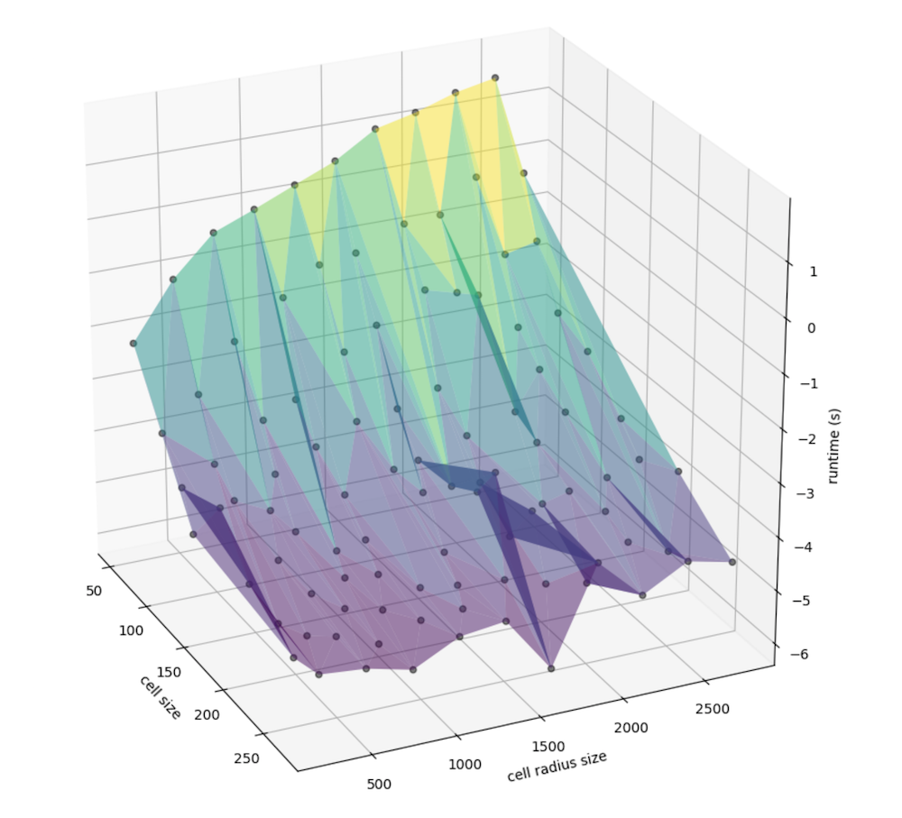
We can better examine the nuance in slope by taking the log of runtime, since there is a nonlinear relationship that may be present:

Similarly, we can view the relationship between window size specifically (instead of that, factored by the cell size) and the cell size (meters, again) with runtime:

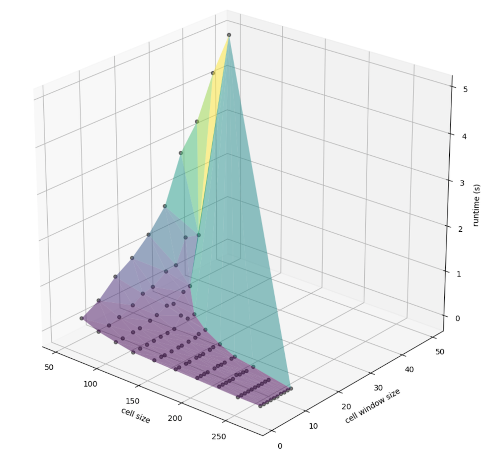
Again, more nuance is visible when taking the log of runtime (in seconds), again:

Exploring the relationships

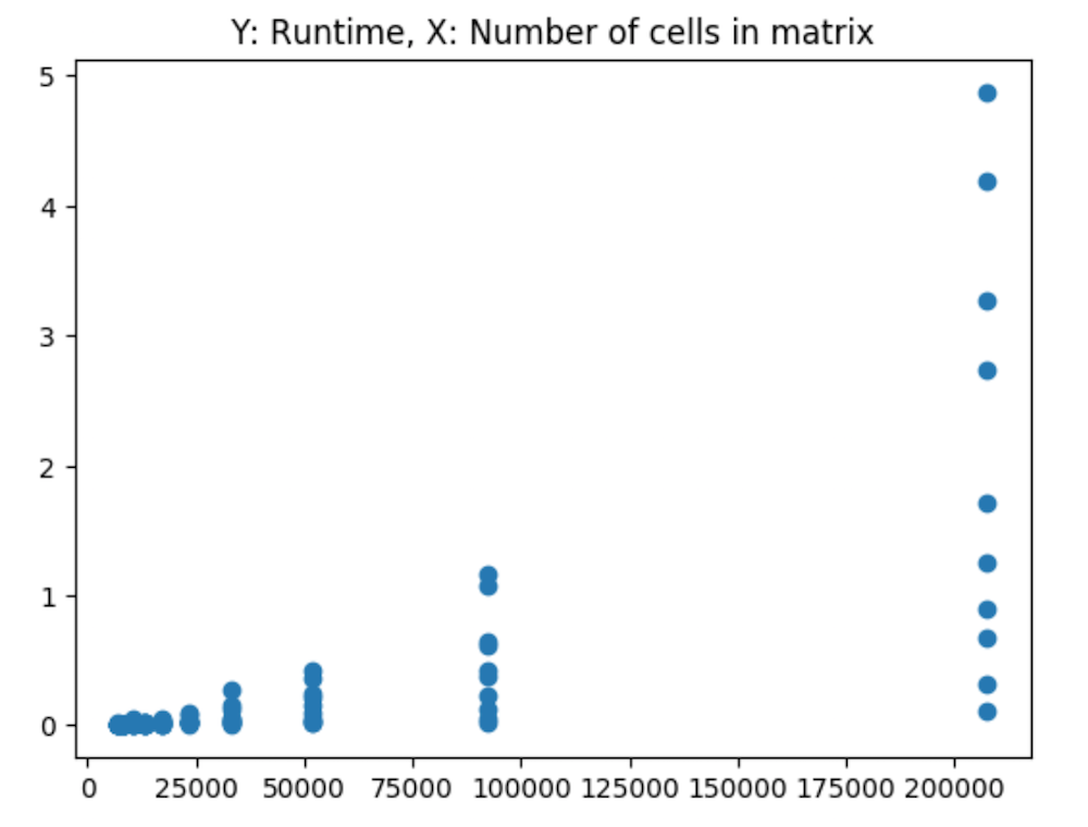
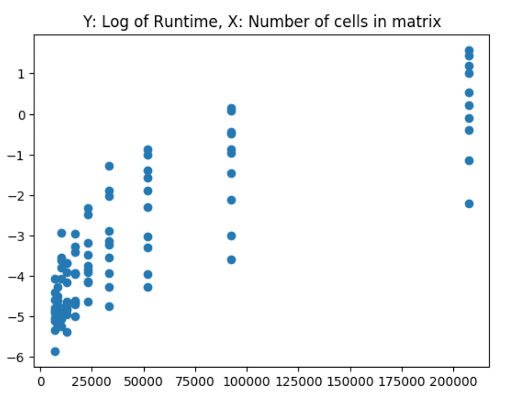
As we can see from these 3-dimensional plots, an consolidated peak is clear. First, let’s look at just the number of cells in the matrix (the number of columns times the number of rows), we can see the exponential increase in cells corresponding with what appears to be a non-linear increase in runtime:

And the log of runtime:

These are calculated via:

res = df.cell_count * df.cells_window
p = np.polyfit(res, df.runtime, 2)
pf = np.poly1d(p)

# Such that the results can be plotted like so:
plt.title('Y: Runtime (s), X: Cell count * cell window')
plt.scatter(res, df.runtime)
sres = sorted(res)
plt.plot(sres, [pf(v) for v in sres], color='red')
plt.show()

Given this relationship, and the clustering along each value on the x axis, I then propose an alternative method, in which we interact the 2 variables use for the x and y axis in the 3d plots earlier. That is, I factor cell radius by cell size to attempt to see how this interaction relates to runtime in seconds.

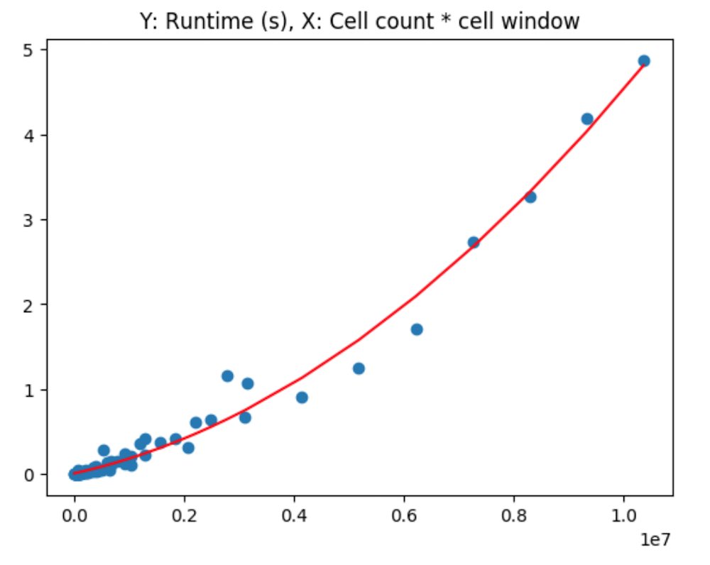
From this, it is clear at this point that a non-linear relationship exists, between the factor of the cell window size and the number of neighboring cells being considered.

Utilizing the observed relationship

Awareness of this can help determine cell size - window radius balance before initializing a run. Using the relationship codified in pf via np.poly1d in the above code snippet, we can instead do this:

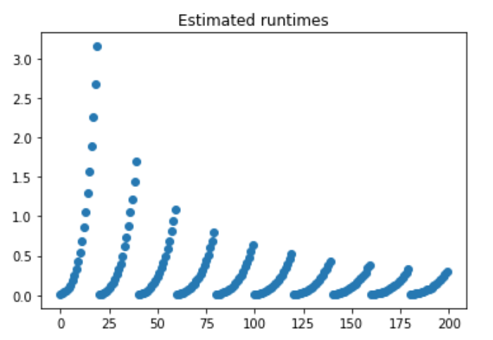
The relationship that we computed for the polynomial can be revealed from this function, such that the method defined prior, pf, is a polynomial comprised of:

poly1d([3.08936507e-14, 1.42656915e-07, 9.32530383e-03])

What we see here are estimated runtimes, with each separate slope representing a larger and larger cell size. The larger the cell size, the less number of cells are needed to create a satisfactory window. Thus, the rate of increase is dampened.

From these results, setting a balancer that is triggered when encountering a time threshold (say, 2 or 3 seconds), may be sufficient for addressing performance concerns regarding model execution runtime.