Introduction
Note that the full notebook for this post is held as a Gist on Github, here.
peartree is useful for converting GTFS schedule data into a network graph. It was, in many ways, inspired by OSMnx, which is a tool that converts OpenStreetMap network data to NetworkX graphs. You can read more about OSMnx, here.
This post shows how to use both tools to create a joint network graph that contains both walk (or drive) network data (from OSM, via OSMnx) as well as transit data from a transit operator’s GTFS feed parsed with peartree.
Dependencies
We will be using peartree version 0.6.1, NetworkX version 2.2, matplotlib version 3.0.2, and OSMnx version 0.8.2.
For the purposes of this example, we will be using the GTFS feed for New Orleans. You can download the latest GTFS feed from New Orleans’ Regional Transit Authority, here.
Extracting the transit graph
Generate the transit graph as you would any peartree graph.
First, get the representative feed:
feed = pt.get_representative_feed('nola_gtfs.zip')Then, pick a target time to extract as a graph (in this case we will do peak hour from seven to nine in the morning.
start = 7 * 60 * 60
end = 9 * 60 * 60
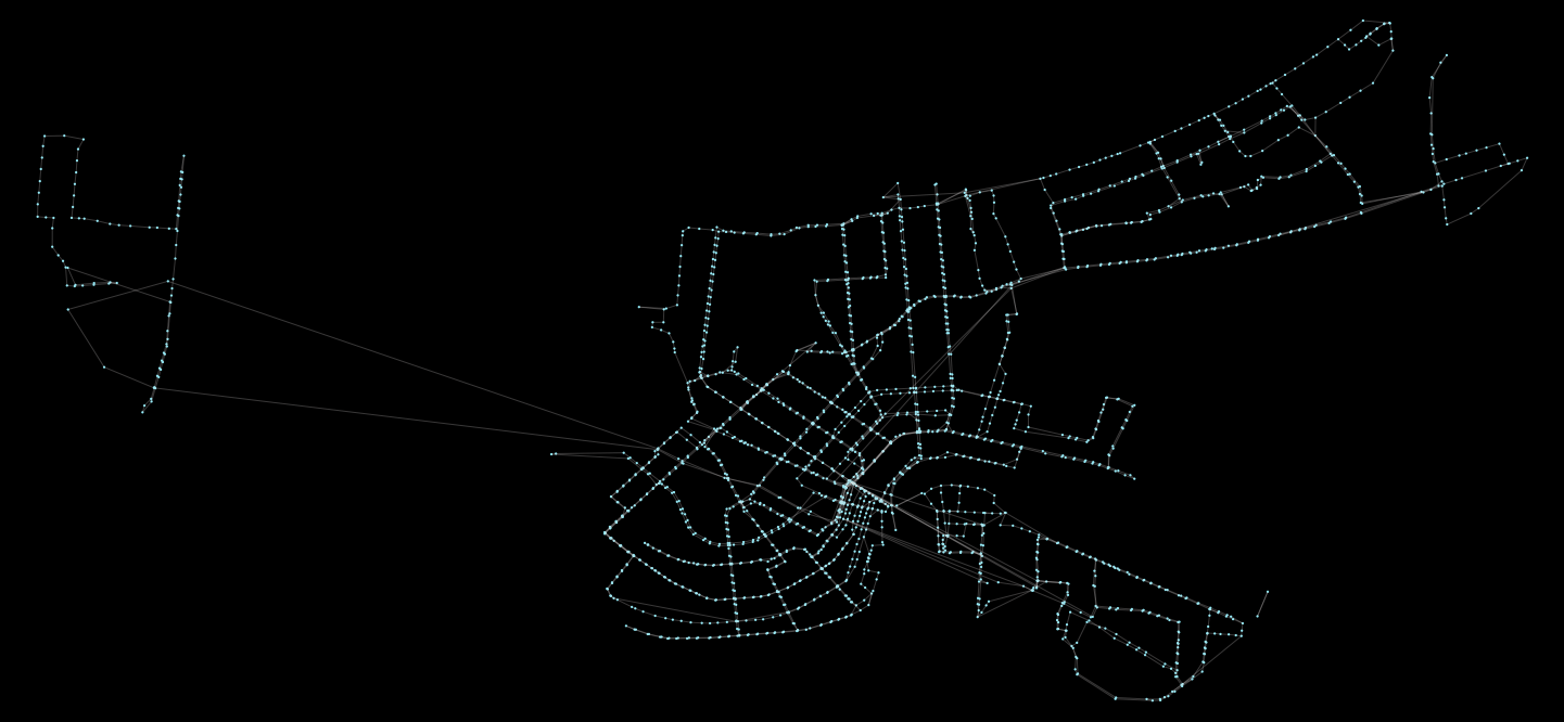
%time G = pt.load_feed_as_graph(feed, start, end)We can view the results like so:
pt.plot.generate_plot(G)This will generate the following graphic:
Generating the walk network
The walk network is also as straightforward as using OSMnx’s standard pattern. In this case, though, we first need a boundary. Let’s use the one that is the coverage area of the transit network. We can get that from the graph we just created. Let’s use a few Shapely operations to help accomplish this:
import geopandas as gpd
from shapely.geometry import Point

# We need a coverage area, based on the points from the
# New Orleans GTFS data, which we can pull from the peartree
# network graph by utilizing coordinate values and extracting
# a convex hull from the point cloud
boundary = gpd.GeoSeries(
    [Point(n['x'], n['y']) for i, n in G.nodes(data=True)]
    ).unary_union.convex_hull
With that result, we can use the new polygon to query OSM for the walk network data to construct a NetworkX graph with:
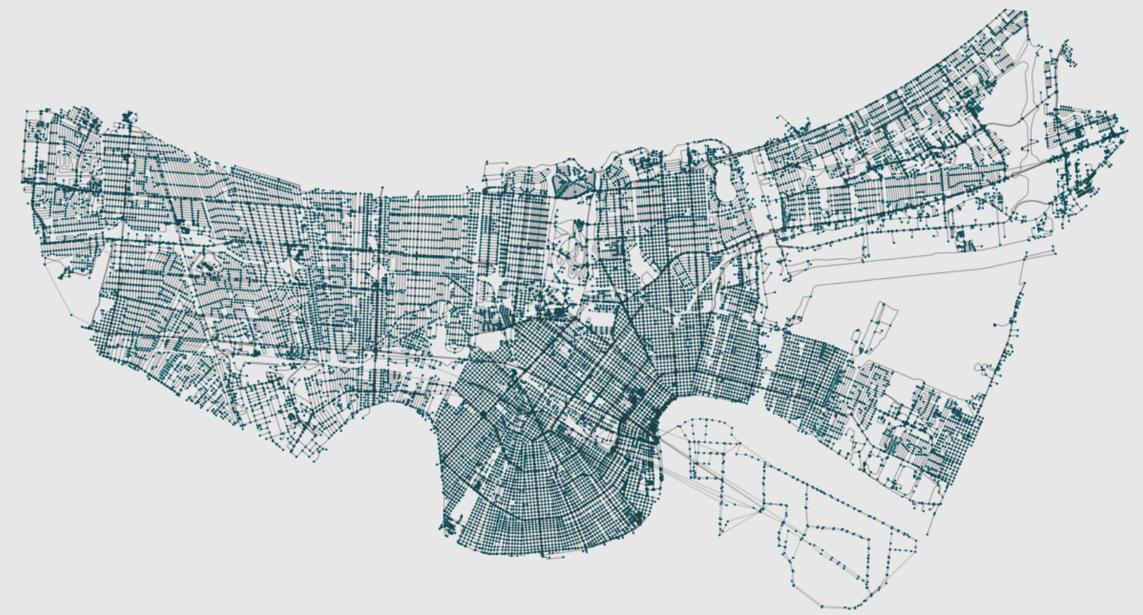
# Pull in the walk network with OSMnx
%time Gwalk = ox.graph_from_polygon(boundary, network_type='walk')
Once again, let’s plot our new graph. We can use OSM to help us do this:
# Visually inspect (takes a minute or two)
ox.plot_graph(Gwalk)
Merging the two graphs
Now comes the fun part; let’s merge the two graphs together. First let’s observe the structure of the two graphs edges:
# Note the edge structure of the peartree graph
list(G.edges(data=True))[0]
# ('9E6AA_10', '9E6AA_5314', {'length': 71.0, 'mode': 'transit'})

# ...and that of the OSMnx graph
list(Gwalk.edges(data=True))[0]
# (115998720,
#  116012585,
#  {'highway': 'residential',
#   'length': 96.733,
#   'name': 'Lane Street',
#   'oneway': False,
#   'osmid': 12703799})
Since peartree represents edge length (that is the impedance value associated with the edge) in seconds; we will need to convert the edge values that are in meters into seconds:
walk_speed = 4.5  # about 3 miles per hour

# Make a copy of the graph in case we make a mistake
Gwalk_adj = Gwalk.copy()

# Iterate through and convert lengths to seconds
for from_node, to_node, edge in Gwalk_adj.edges(data=True):
    orig_len = edge['length']

    # Note that this is a MultiDiGraph so there could
    # be multiple indices here, I naively assume this is not
    # the case
    Gwalk_adj[from_node][to_node][0]['orig_length'] = orig_len

    # Conversion of walk speed and into seconds from meters
    kmph = (orig_len / 1000) / walk_speed
    in_seconds = kmph * 60 * 60
    Gwalk_adj[from_node][to_node][0]['length'] = in_seconds

    # And state the mode, too
    Gwalk_adj[from_node][to_node][0]['mode'] = 'walk'
We can now check that we do indeed have the original length value preserved:
# Ensure that we now have both length values (and
# thus an updated edge schema)
list(Gwalk_adj.edges(data=True))[0]
# (115998720,
#  116012585,
#  {'highway': 'residential',
#   'length': 77.3864,
#   'mode': 'walk',
#   'name': 'Lane Street',
#   'oneway': False,
#   'orig_length': 96.733,
#   'osmid': 12703799})
Now we need to update the nodes. All nodes need to have a boarding cost. We can ensure that all OSMnx nodes have a boarding cost of 0 by simply assigning that value to each of them:
# So this should be easy - just go through all nodes
# and make them have a 0 cost to board
for i, node in Gwalk_adj.nodes(data=True):
    Gwalk_adj.node[i]['boarding_cost'] = 0
Now that the two graphs have the same internal structures, we can load the walk network onto the transit network with the following peartree helper method:
# Now that we have a formatted walk network
# it should be easy to reload the peartree graph
# and stack it on the walk network
start = 7 * 60 * 60
end = 9 * 60 * 60

# Note this will be a little slow - an optimization here would be
# to have coalesced the walk network
%time G2 = pt.load_feed_as_graph(feed, start, end, existing_graph=Gwalk_adj)
Clean up steps
Unfortunately, there’s a few issues that can arise when performing this merge. I intend on eventually working out the kinks - but in the meantime the main thing to check for is hanging nodes. When performing the stacking operation of adding the walk network to the transit network, some nodes can become isolated (attached to nothing else). These isolated subgraphs with no edge count can be removed safely. The following outlines a pattern to use to do so:
# This is an issue that needs cleaning up
# slash I need to look into it more
# but some nodes that should have been
# cleaned out remain
print('All nodes', len(G2.nodes()))
bad_ns = [i for i, n in G2.nodes(data=True) if 'x' not in n]
print('Bad nodes count', len(bad_ns))

for bad_n in bad_ns:
    # Make sure they do not conenct to anything
    if len(G2[bad_n]) > 0:
        # This should not happen
        print(bad_n)

    else:
        # So just drop them
        G2.remove_node(bad_n)
Conclusion
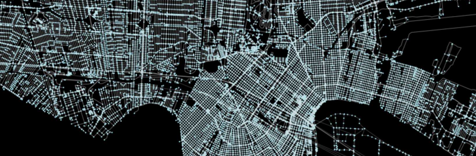
And there you have it - following those simple steps should be sufficient to generate a combined graph. We can now view it as though it were any other peartree graph:
pt.plot.generate_plot(G2)