On-street Open Parking Data

Introduction

I was reading a recent blog post on converting curb parking regulation data in Calgary into CurbLR format (linearly referenced data). I wanted to take a stab at performing this conversion myself. Since I live in Oakland, California, I wanted to pull available data for that municipality. Unfortunately, I was not able to find any pre-existing curb data that Oakland had available.

I’d recently been approached about street sweeping data in Sacramento. I was curious if Sacramento had decent parking data, which they do. They have a large point data set which appears to indicate the state of each parking spot throughout what appears to be the central business district. In this post I make some cursory observations about this data as I pull it down and process it.

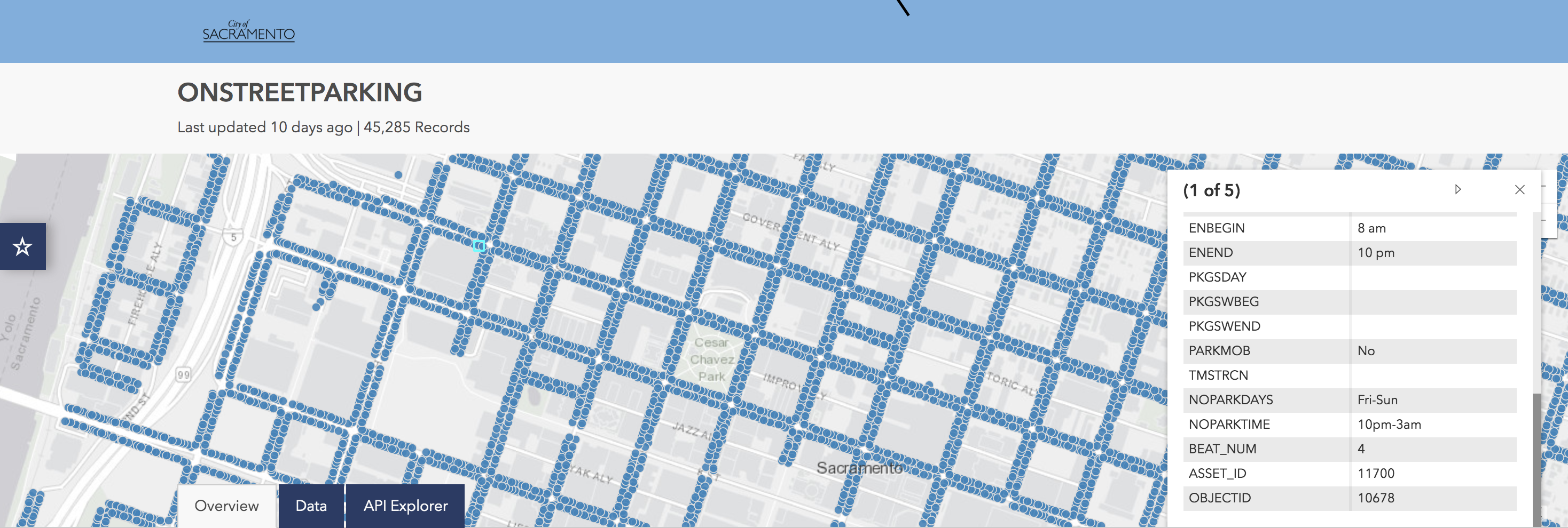
Above: Shot of the parking point data in the Open Data Portal that Sacramento has.

Loading the data

Unfortunately, there is no data dictionary for this data.

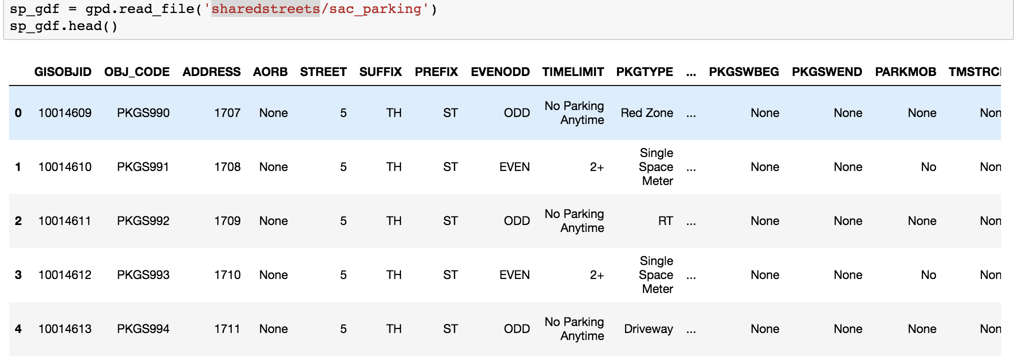
Loading the shape file representing all points into a notebook shows that there are a host of columns that are unexplained.

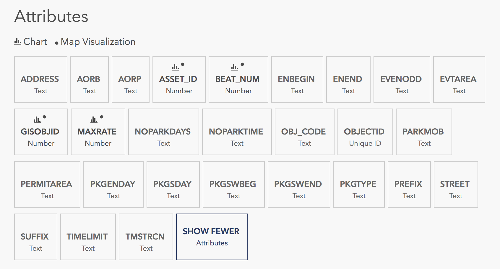
This is also shown in the Open Data Portal. Unfortunately, there is not any additional explanation for what these column names mean.

I tried to work through the columns but ultimately could not figure out what the following columns mean:

# Unfortunately, I can't find a data dictionary so dropping all columns
# that I am unable to determine what they represent
unknown_cols = [
    'GISOBJID',
    'OBJ_CODE',
    'AORB',
    'EVENODD',
    'BEAT_NUM',
    'ASSET_ID',
    'OBJECTID',
    'PARKMOB',
]

There are also a few columns that I dump because I figure I do not need them for this work.

# Also drop columns that are unwanted for the purposes
# of this exercise
unwanted_cols = [
    'ADDRESS',
    'STREET',
    'SUFFIX',
    'PREFIX',
]

I go ahead and trim these columns out, as shown below:

# Given the columns we explicitly want to reduce, produce a subset of
# columns that are just those that we intend to keep
exempt_cols = unknown_cols + unwanted_cols
keep_cols = [c for c in sp_gdf.columns if c not in exempt_cols]

Now, I rename the remaining column names with the column names that better highlight what I think they mean. Again, this is all just me examining the data and guessing what the column is. If there is a data dictionary somewhere, I would be very interested in it!

# Rename them to get them out of the 10 character limit from their Shapefile
# source format
rename_dict = {
    'TIMELIMIT': 'time_limit',
    'PKGTYPE': 'space_type',
    'AORP': 'style',
    'PERMITAREA': 'permit_zone',
    'MAXRATE': 'max_rate',
    'EVTAREA': 'event_zone',
    'PKGENDAY': 'enforcement_days',
    'ENBEGIN': 'enforcement_time_start',
    'ENEND': 'enforcement_time_end',
    'PKGSDAY': 'sweeping_days',
    'PKGSWBEG': 'sweeping_time_start',
    'PKGSWEND': 'sweeping_time_end',
    'TMSTRCN': 'details',
    'NOPARKDAYS': 'not_allowed_days',
    'NOPARKTIME': 'not_allowed_timeframe'
}

# Make sure that the date contains all geometries we need
rename_col_vals = list(rename_dict.keys()) + ['geometry']
assert set(list(rename_dict.keys()) + ['geometry']) == set(keep_cols)

# Rename columns to their more readable counterparts
sp_gdf = sp_gdf[keep_cols].rename(columns=rename_dict)

Pruning the spatial data

At this point there appear to be some stray points that fall well outside of the central business district.

What I want to do is just get the largest cluster and focus on that.

from shapely.geometry import MultiPolygon

# There are some extraneous small points so clean them out
sp_gdf.crs = {'init': 'epsg:4326'}
ea_temp_gdf = sp_gdf.to_crs(epsg=2163)
ea_uu = ea_temp_gdf.buffer(50).unary_union
assert type(ea_uu) == MultiPolygon 

# Just get the biggest set
ea_main = max(ea_uu, key=lambda x: x.area)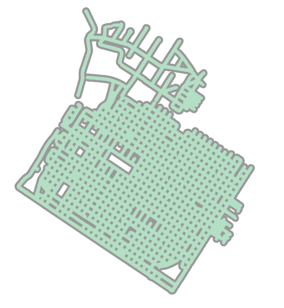

Above: This produces the following subset cluster.

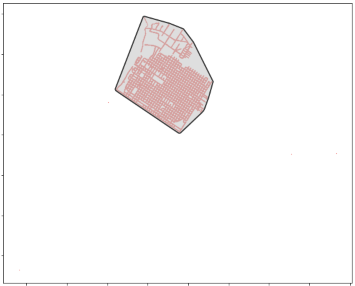
Above: We can see how this portion (circled in black above) is most of the points and there are a small smattering of points elsewhere near the site. I do not know why those other points are included, but I am ignoring those for now.

Above: This is the subset alone shown of just the points in the central business district in Sacramento.

Exploring street sweeping data

I set up the following filters to just limit to data points that have street sweeping attributes:

# Look at just street sweeping data
m1 = sp2_gdf['sweeping_days'].isnull()
m2 = sp2_gdf['sweeping_time_start'].isnull()
m3 = sp2_gdf['sweeping_time_end'].isnull()
m = ~m1 & ~m2 & ~m3
sweep_gdf = sp2_gdf[m]

print(f'trimmed from {len(sp2_gdf)} to {len(sweep_gdf)} geometries')
# trimmed from 45281 to 7630 geometries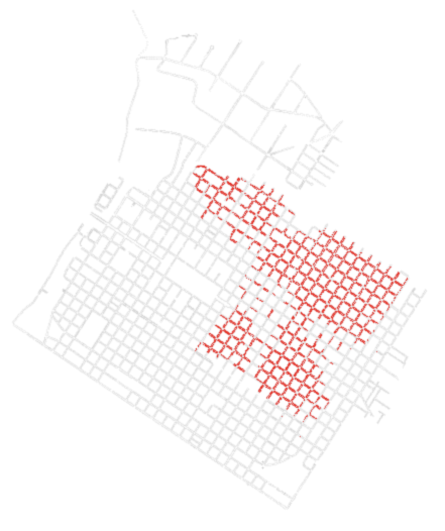

Above: This removes about 80% of all the points. Plotting the points with street sweeping data in red shows that it appears that this data is only available in the north east portion of the city. I doubt that street sweeping is only available in that portion of the city and would like to know why that information appears to be incomplete.

Testing map matching with SharedStreets

At this point I wanted to simply observe how SharedStreets handled this point data. Since the blog post example from Calgary included segment data published by the city, matching that to segments to see coverage areas “made sense.” In this case, I just have points. What will SharedStreets do?

To start, I take just a small arbitrary subset of this data that has street sweeping information.

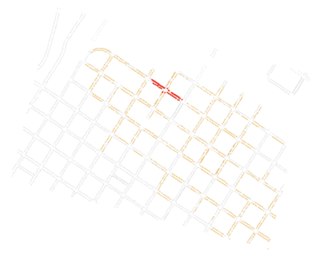
Above: The small subset is in red. The street sweeping data is in orange.

I can go ahead and export this small exploratory subset of 2 blocks of point data to a GeoJSON.

sweep_gdf_sub['geometry'].to_file('sharedstreets/test_points.geojson', driver='GeoJSON')

Now, in the terminal, I can run the node library shst that SharedStreets distributes and run the map matching algorithm on my GeoJSON of point data.

shst match test_points.geojson --search-radius=20 -o=points --best-direction

I can now read the resulting data back in and plot it.

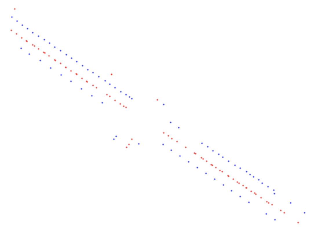
Above: The original points are in blue (points on both sides of street). The matched data is in red. Note that the matched data falls along the centerline.

So, what happened to the street sides as they were represented in the original point data? The returned SharedStreets matched GeoJSON includes attributes indicating whether the point is on the left or the right side of the street and the direction of the street.

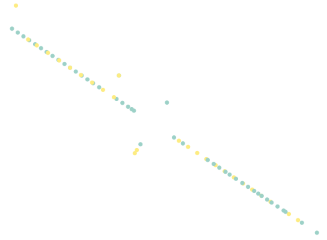
Above: Coloring the map matched data where yellow is left and green is right. This shows how the different sides of the road are represented while the map matched points fall in the centerline.

Next steps

This was just the earliest work on finding some data, cleaning it, and map matching the geometries. Next up; I’ll need to learn more about the CurbLR specification (which it sounds like is still in flux) and figure out how to link points together that have the same attributes to create actual segments that can be paired with SharedStreets to show what portions of a curb are designated for certain uses.