Introduction

Conveyal offers an open source GTFS editing tool. You can read about it here. The tool allows for new lines to be drawn and described as a collection of stops and a line (shape) with operational characteristics held as metadata. (Note: This information is out of date - see comments at the bottom of this post for details.)

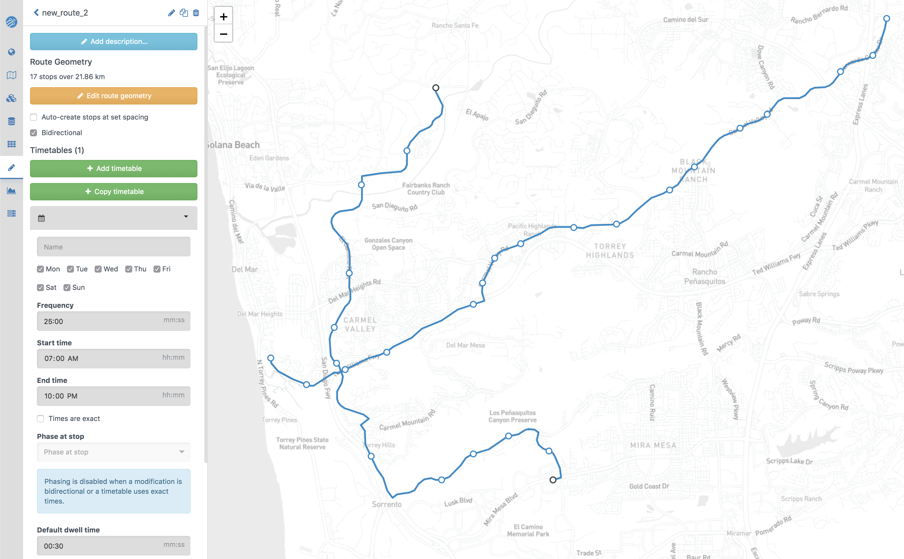
Above is an image of what the interface looks like.

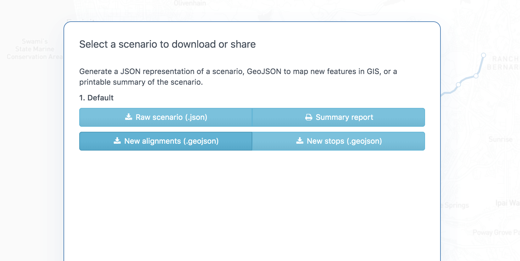
This tool allows for export of the lines that are drawn and the stops that are added in a summary JSON format. The notes below demonstrate how to take this information and convert it to 2 structured summary data frames: a stops dataset and an edges dataset.

With these two converted datasets, addition to a network graph is easy. The format produced can be passed directly into peartree for example, so that new, custom transit can be added directly from Conveyal’s open source tools and into a peartree network graph. This can be useful for lightweight, notebook based exploration of how a new transit line interacts with an existing network (held as GTFS), for example.

Reading in the data

To start, let’s just use geopnadas easy read operation to read in the two GeoJSONs and hold them in data frame form.

import geopandas as gpd

alignments_gdf = gpd.read_file('conveyal/test_alignments.geojson').to_crs(epsg=2163)
stops_gdf = gpd.read_file('conveyal/test_stops.geojson').to_crs(epsg=2163)

We can plot the results easily.

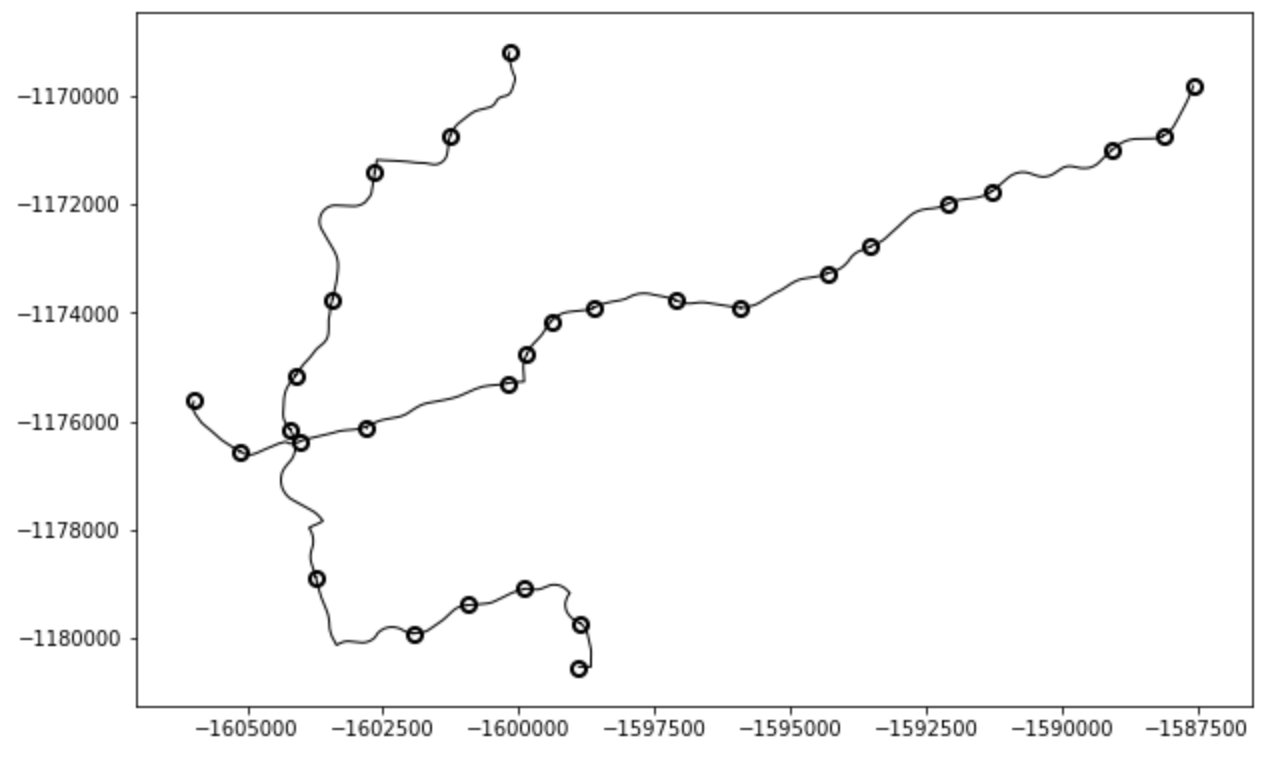
Above: Results of plotting the lines and stops. As we an see, it looks comparable to the results viewable in the transit editing portion of the app.

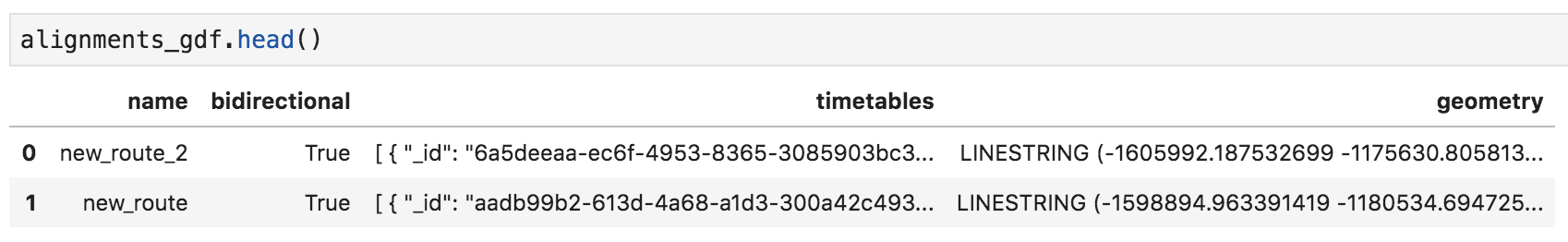
Note that the alignments data frame holds the contents of the timetable attributes as a stringified array. See the above log of the alignment data table to see what that looks like.

sorted_stops_gdf = stops_gdf.groupby('name').apply(lambda x: x.sort_values(by='distanceFromStart').reset_index(drop=True)[['distanceFromStart', 'geometry']])

For stops, we just want the distance measure and the geometry. We can then group by the name of each route. We will use these to pair with the alignments.

Pairing the stops

We need to find which stop goes where on the line. We need to determine how long each subsegment is. This method is not necessarily the bus, but works if we rely on the stops data being returning from Conveyal to be vetted in the sense that the stops do indeed exist along the route.

Indeed, in this method the stops that are placed too far off the route (should not happen with default output) would get dropped. An alternative would be to use a more advanced line matching pattern to pair the stops to the line.

In this case, we are assuming that this has already occurred and we just want to subdivide the route into separate lines for each segment. We are already working in a meter based projection so division of the route into segments with a small buffer avoids any minor offsets and provides a “good enough” measure for each segment distance.

route_names = alignments_gdf['name'].tolist()
route_name = route_names[0]

A note before showing the full logic: We are at this point just working with one alignment. We simply need to apply the following logic to all route names to be get the edges and nodes for each new line.

from shapely.geometry import MultiPoint
from shapely.ops import split

buffer_size = 10

mask = alignments_gdf['name'] == route_name
alignment_row = alignments_gdf[mask].squeeze()

related_stops = sorted_stops_gdf.loc[route_name]
stop_geoms = related_stops['geometry'].tolist()
stop_geoms = MultiPoint(stop_geoms).buffer(buffer_size)

route_geom = alignment_row['geometry']

split_line = split(route_geom, stop_geoms)
split_line = [l for l in split_line if l.length > buffer_size * 2]

We can color the plot to show each segment and how the stops were separators.

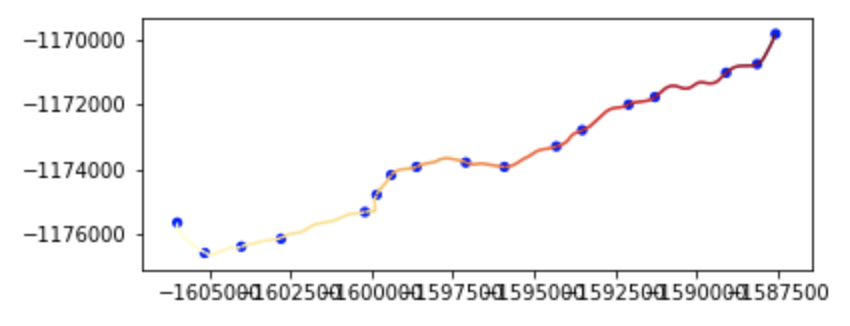
ax = gpd.GeoSeries(split_line).plot(cmap='YlOrRd')
gpd.GeoSeries(stop_geoms).buffer(150).plot(ax=ax, color='blue')

Above: Segments for a single route plotted.

Cleaning timetable metadata

As shown earlier, the alignment data is stringified. First, we should parse it for the target alignment.

import json

timetables = json.loads(alignment_row['timetables'])
timetable = timetables[0]
seg_speeds = timetable['segmentSpeeds']

assert len(split_line) == len(seg_speeds)

Segment extraction for time is a function of the indicated speed for that segment, paired with the length calculated for that segment. Speeds are in kilometers and the length is in meters, so a 1000x conversion is also applied.

segment_times = []
for line, speed in zip(split_line, seg_speeds):
    len_meters = line.length
    len_kms = len_meters / 1000
    hrs_elapsed = len_kms / speed
    secs_elapsed = hrs_elapsed * (60 * 60)
    segment_times.append(secs_elapsed)

I also rolled in the dwelling times into the edge costs and shifted the cost to the following cost segment. I assume if you arrive at a destination you should not have to wait that additional amount of time since, at that point, you can just deboard the vehicle.

# Default dwell times as all being the same
num_stops = len(related_stops)
dwell_times = [timetable['dwellTime']] * num_stops

# But if custom ones present, use those instead
if 'dwellTimes' in timetable:
    assert len(timetable['dwellTimes']) == num_stops
    dwell_times_override = []
    for odt, ndt in zip(dwell_times, timetable['dwellTimes']):
        if ndt:
            dwell_times_override.append(ndt)
        else:
            dwell_times_override.append(odt)
    dwell_times = dwell_times_override
    
# Ignore the last stop dwell time and move the dwell times
# into each of the preceding segment's times
segment_times = [st + dt for st, dt in zip(segment_times, dwell_times[:-1])]

We now have edge costs. We can get the stop ids paired with each edge and create a summary data frame:

import pandas as pd

stop_ids = [f'{route_name}_{i}' for i in related_stops.index]

froms = stop_ids[:-1]
tos = stop_ids[1:]
assert len(froms) == len(tos)
assert len(tos) == len(segment_times)

edges_df = pd.DataFrame(
    [x for x in zip(froms, tos, segment_times)],
    columns=['from_stop_id', 'to_stop_id', 'edge_cost'])

edges_df.head()

Nodes are easy at this point as well. We have the stop latitude and longitude already from the geometry data and just need to convert it to ESPG 4326 (web mercator) projection.

We also need to add headways. This is available as a single metadata parameters we can pull out. In the future, an improvement could be to provide a better function for calculating the average wait time. For example, for certain types of routes people might intentionally schedule their arrivals and thus wait times might want to be modeled as less than half the wait time.

nodes_df = pd.DataFrame(
    [(p.x, p.y) for p in related_stops.to_crs(epsg=4326)['geometry']],
    columns=['stop_lon', 'stop_lat'])

assert len(stop_ids) == len(nodes_df)

nodes_df['stop_id'] = stop_ids

Conclusion

This operation can now be run for each alignment name to produce the necessary edges and nodes data frames that are used to create graph edges.

You can see how these are used in the peartree library by viewing the synthetic.py file and seeing how it consumed new summary nodes and edges data frames.

Here is nodes data frame generation.

Here is edges data frame generation.

Update

• An update was requested by Anson at Conveyal. Per Anson: “For clarity, it might be good to specify that [I was] using the scenario editing features of Conveyal Analysis. The “data tools ui” [that was referenced] is actually a separate codebase now under IBI’s control.” More on that can be found, here.