Cost estimating synthetic edges

Introduction

Intent is to document performance cost of adding synthetic node to edge leafs. Why would one do this? One example use case is to create summary walk access edges and nodes along end of remote our outlying transit service areas.

Instead of assigning all accessible jobs to final transit stop, desire might be to “string out” jobs linearly along synthetic walk network edges that extend out, one after another, from target transit nodes.

Such a method would model walk access from transit node to jobs. Also would avoid unrealistic and oversized “boost” in jobs access the moment you are able to reach this outlying transit node.

This seems ideal from a clean modeling perspective, but what are the costs of adding synthetic nodes to a representative network? Synthetic nodes add to the complexity of the network and can slow down pathfinding operations. This post creates a simple example model and demonstrates the increased cost of addition of synthetic nodes.

Set up an example graph

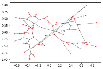
For the purpose of this post, instead of using a real transit network, let’s just create an example one using the random_lobster algorithm available with networkx. It’s a close enough approximation, creating a main “spine” and some branching paths out from that core trunk.

import networkx as nx
import random

backbone_size = 500

G = nx.random_lobster(backbone_size, 0.9, 0.9)

# Give each node some random weights
for fr, to, e in G.edges(data=True):
    G.edges[fr, to]['weight'] = round(random.random() * 100)

# Make a directed graph (all nodes connect in both directions for now)
G = G.to_directed()

# Also make a copy of the original for reference layer
# since we are going to do some modifications
G_orig = G.copy()

Drawing the graph will result in something like the following:

Summarize existing network

Before modifying the network, capture aspects of the network as they currently exist. We will use these as references for evaluating performance before and after.

node_ids_to_consider = list(G.nodes())

print(len(node_ids_to_consider), 'nodes to consider')
# 1422 nodes to consider

The above operation gets us the ids of the nodes that presently are in the original graph.

end_nodes = []
for nid in node_ids_to_consider:
    l = len(list(G.neighbors(nid)))
    if l == 1:
        end_nodes.append(nid)
        
print(len(end_nodes), 'end nodes found')
# 474 end nodes found

The above gets us the ids of the nodes on the ends of these leafs branching out from the main spine of the network graph.

start_num_new_nodes = max(node_ids_to_consider)

print('current largest node id is', start_num_new_nodes)
# current largest node id is 1421

Finally, we get the largest node id so that when we begin to modify the graph, we do not override any existing nodes.

Adding synthetic nodes to the graph

Now let’s add new nodes to the graph. Let’s add 10 per each leaf nodes that we identified. We can imagine that this would allow the graph to model walk access to some target metric (like jobs) at, say, 2 minute increments and thus model walk access to this resource within a 20 minute walk of the transit station (about a mile).

We can modify the graph now by iterating through and adding those 10 nodes stretching out from each of the prior identified edge nodes.

num_nodes_to_add_per = 10

last_num_used = start_num_new_nodes
for nid in end_nodes:
    last_used_for_leaf = nid
    for i in range(num_nodes_to_add_per):
        new_nid = last_num_used + 1
        
        w = 5
        
        G.add_node(new_nid)
        G.add_edge(nid, new_nid, weight=w)
        
        last_num_used = new_nid
        last_used_for_leaf = new_nid

Evaluating modification impacts

We can now calculate how much the graph changed before and after the addition of synthetic nodes.

new_len = len(list(G.nodes()))
old_len = len(node_ids_to_consider)

diff = new_len - old_len
print(diff, 'new nodes added')
# 4470 new nodes added

pct_increase = (new_len / old_len) * 100
print('network increased in size by', round(pct_increase, 2), 'percent')
# network increased in size by 434.08 percent

Comparing performance

We can see what run time looked like originally, by calculating shortest path to all nodes from each node in the original graph and how that increases when the graph is then updated.

First let us look at the performance of the original graph:

%%time
for nid in node_ids_to_consider:
    nx.single_source_shortest_path_length(G, nid)

# CPU times: user 20.7 s, sys: 20 ms, total: 20.7 s
# Wall time: 20.7 s

Now let’s look at the performance of the new, modified graph:

%%time
for nid in node_ids_to_consider:
    nx.single_source_shortest_path_length(G_orig, nid)

# CPU times: user 5.31 s, sys: 10 ms, total: 5.32 s
# Wall time: 5.35 s

That’s about 386% longer on a network that is 434% larger. Very roughly, a 4x increase in the number of nodes here corresponded with a similar increase in the runtime for calculating shortest paths.

While there are a variety of optimizations that can be made on graph access calculation (as well as not using a pure-python graph implementation like NetworkX), the fact stands that mutating the original graph can introduce some significant performance-related costs when attempting to model path access for leaf edge end nodes (for example).