Hierarchical clustering of trip traces

Introduction

The intent of this post is to demonstrate how one might use a hierarchical system (in this case, S2 cells) to summarize discrete agent trips in a summary fashion that attempts to address privacy concerns by agglomerating sparse trace patterns at higher levels of aggregation.

That is, by reducing the accuracy with more coarse approximations where a plurality of location data is lacking, trace attributes can be preserved and summarized over larger areas where data volume is deemed sufficient for representation.

Details

This post outlines first how to create some synthetic trace data to work with, then how to execute the anonymization outlined in the above. Note that the intent is to broadly capture how this might be done, not to present this as a de facto method that should be replicated in a real world use case. Most importantly, I want to highlight the opportunity for there to be a function “inserted” that would allow for the threshold that determines sufficiency of data density to be calculated dynamically (and to be managed as a user-defined input).

What might be an acceptable level of accuracy and aggregation for one use case may not be appropriate for another.

Creating synthetic data

To create a synthetic trace dataset, I used this trip simulator and followed the README, generally.

First, I pulled down a target city’s PBF. In this case, I pulled down St. Louis, Missouri. I trimmed the extract to a subset of the whole metro area, so as to just simulate traffic around the downtown area.

curl https://s3.amazonaws.com/metro-extracts.nextzen.org/2018-05-19-13-00/saint-louis_missouri.osm.pbf -o stlouis.osm.pbf
osmium extract -b "-90.300896,38.592407,-90.176938,38.675982" stlouis.osm.pbf -o ./stl.osm.pbf -s "complete_ways" --overwrite

I then npm installed OSRM, the OpenStreetMap routing engine and processed the road graph.

./node_modules/osrm/lib/binding/osrm-extract ./stl.osm.pbf -p ./node_modules/osrm/profiles/foot.lua;
./node_modules/osrm/lib/binding/osrm-contract ./stl.osrm

Finally, I ran a configured trip-simulator run on this subset of the road network with 100 agents to create a series of traces represented in the output trips.json file.

trip-simulator \
  --config scooter \
  --pbf stl.osm.pbf \
  --graph stl.osrm \
  --agents 100 \
  --start 1563122921000 \
  --seconds 21600 \
  --traces ./traces.json \
  --probes ./probes.json \
  --changes ./changes.json \
  --trips ./trips.json

Aggregating trip traces to hierarchical summary format

At this point, I now have trace data simulated for a given period of time. I want to take this trace data and aggregate the trips so that they exist at a level of detail that avoids exposing personal information based off of a threshold that is customizable to the use case.

To start, let’s read in the data as a GeoDataFrame in Python.

import geopandas as gpd
import json

# read in the trips file
with open('trips.json') as f:
    trips = [json.loads(l) for l in f]

# for each route, generate a data frame and stack
# on top of preceding converted routes
gdf = None
for t in trips:
    gdf_temp = gpd.GeoDataFrame.from_features(t['route'])
    gdf_temp['vehicle_id'] = t['vehicle_id']

    if gdf is None:
        gdf = gdf_temp
    else:
        gdf = gdf.append(gdf_temp)

We can observe the result of this by plotting the data. In blue is the individual point data and in red are the line strings that are created by converting each of these traces to complete line string-traced trips.

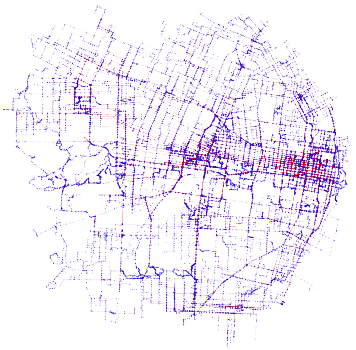
The darker red lines have more trips associated with those segments.

Pairing traces with S2 cell

For each trace point, we want the smallest S2 cell associated with it. From that cell, we then want all that S2 cells parent cells (so from the highest zoom all the way out to the maximum zoom).

To do this, we will use a library s2sphere that facilitates working with the concept of the S2 cell hierarchy.

import s2sphere

p_sets = []
for pt in gdf_ll.geometry:
    ll = s2sphere.LatLng.from_degrees(pt.y, pt.x)
    p = s2sphere.CellId.from_lat_lng(ll)
   
    # there are 30 zoom levels for s2 cells
    assert p.MAX_LEVEL == 30
    assert p.level() == 30

    # create a list of each zoom's parent
    # s2 ids from max zoom all the way out
    p_set = []
    for i in range(31):
        p_set.append(p.id())
       
        if p.level() > 0:
            p = p.parent()

    assert len(p_set) == 31
   
    # we want each index to pair with related zoom level
    p_set.reverse()
   
    # add to the column tracker list
    p_sets.append(p_set)

gdf_ll['parents'] = p_sets

Now we can look at each zoom level and see how many values are in each cell. We can create a rule system here that, for each zoom level, if there are enough points, we can assert that this zoom level for a certain S2 cell is “ok” to pass through to the output.

from collections import Counter

gdf_temp = gdf_ll.copy()

# zoom level 22 is equivalent to 4.83 meters square
z_lvl = 0
min_density = 10

while z_lvl <= 22:
    z_lvl_ok = []

    # get parent at given zoom level for each row
    ps = [x[z_lvl] for x in gdf_ll['parents']]
   
    c = Counter(ps)
   
    for p in ps:
        z_lvl_ok.append(c.get(p) > min_density)
       
    gdf_temp[f'z{str(z_lvl)}_ok'] = z_lvl_ok
   
    # increment
    z_lvl += 1

Note that we could also make this logic dynamic where, perhaps, thresholds are lower at lower zooms. For example, even if there is just one trace, we allow it to be rendered at a very coarse level (say, a cell id that is the scale of 100 square miles or something).

Now, each trace point has associated with it a list of parent cells at progressively lower zooms. It also has a register that indicates what zooms it is ok to show this trace at. From this, we can determine what the highest acceptable zoom is, based on the parameter we came up with and injected in the previous section.

eval_cols = []
for c in gdf_temp.columns:
    if c.startswith('z') and c.endswith('_ok'):
        v = c.replace('z', '').replace('_ok', '')
        v = int(v)
        eval_cols.append(v)
eval_cols = sorted(eval_cols)
print('Evaluating columns:', eval_cols)

def get_min_zoom(row, cs):
    min_c = None
    for c in cs:
        col_name = f'z{str(c)}_ok'
        if row[col_name]:
            min_c = c

        # stop on the last/highest true val
        if row[col_name] is False:
            break
    return min_c

min_z = gdf_temp.apply(lambda r: get_min_zoom(r, eval_cols), axis=1)
gdf_temp['min_z'] = min_z

Now we know what the zoom is (and, as a result, the index of the parent cell id from the parent cells list).

Since we have all traces in this GeoDataFrame, we want to know create paths that are based off the highest accepted zoom level for each trace for each unique trip or agent. In this case, we can start by doing this for each agent by using the vehicle_id parameter which identifies each agent’s trips.

def get_path_as_cell_ids(gdf_sub):
    gdf_sub = gdf_sub.sort_values(by='timestamp')

    z_id_list = []
    for i, row in gdf_sub.iterrows():
        nxt_parent = row['parents'][row['min_z']]

        if len(z_id_list) == 0:
            z_id_list.append(nxt_parent)
           
        elif not z_id_list[-1] == nxt_parent:
            z_id_list.append(nxt_parent)

    return z_id_list

path_sets = gdf_temp.groupby('vehicle_id').apply(get_path_as_cell_ids)

# This produces a result that resembles the following:
# vehicle_id
# ADI-1649    [9788770841310265344, 9788770843994619904, 978...
# AKK-3435    [9790626240070156288, 9790626239801720832, 979...
# ALC-5959    [9788773260182159360, 9788773258034675712, 978...

Rendering the result

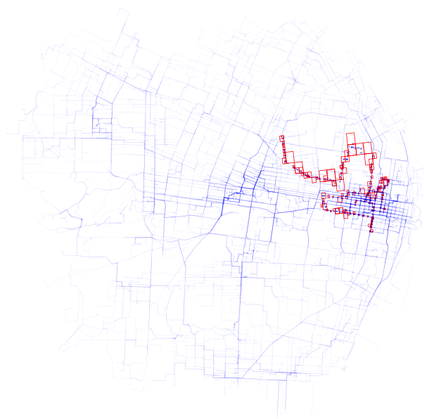
At this point we can render all those trips as their S2 cell representation by converting the S2 cell ids into shapes and plotting those shapes.

def convert_point_to_latlng(p):
    # TODO: terrible hack, see:
    # https://github.com/sidewalklabs/s2sphere/issues/39
    ll = s2sphere.LatLng.from_point(p)
    l = list(map(float, str(ll).split(': ')[1].split(',')))
    return [l[1], l[0]]

# iterate through each path and convert each cell set to a shape
for veh_id, veh_s2_cell_path in sample_veh_paths.items():
    path_as_cell_shapes = []
    for cell_id in veh_s2_cell_path:
        cell = s2sphere.Cell(s2sphere.CellId(cell_id))
        vs = [cell.get_vertex(v) for v in range(4)]
        path_as_cell_shapes.append(
            Polygon([convert_point_to_latlng(p) for p in vs]))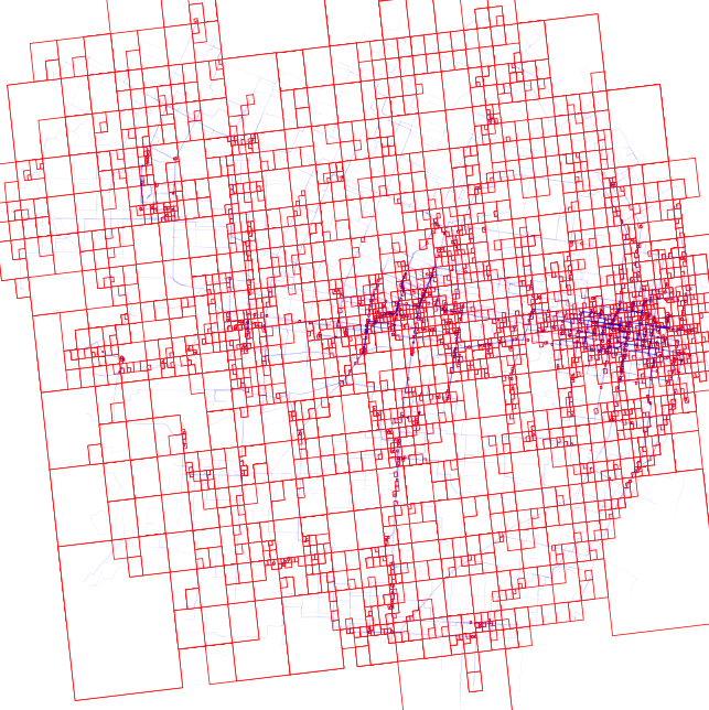

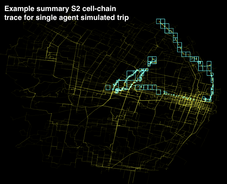
Now, this result can be a bit visually overwhelming. As a result, it may help to just look at how one trip has been converted. Shown is the road network, the trace for a single vehicle id, and the associated S2 cell conversion.

Next steps

This is just a simple aggregation concept. In the end, segments of multiple trips that are common could be agglomerated amongst multiple sources and, from these sources, typical runtimes for that set of S2 cells could be generated.

From this, one might imagine that typical ETAs could be generated from a given S2 cell to another at certain levels and typical traffic patterns associated without needing to sacrifice privacy.

Additional steps, such as anonymizing agent trips or further distilling travel patterns could be pursued. Again, this is just a very high level concept of how one could begin to consider whole trips without risking personally identifiable information.