Introduction

The goal here is to outline a heuristic that will, when given a set of raw gps traces that pass through some target area, and extract a “representative trunk: from that set of paths. That is, we want to know the portion of the traces that most of the traces move through - what that main section is from which all the traces traverse and then branch out.

Example dataset

Here we can start with some synthetic traces such as the ones shown below. These represent traces in and around some target corridor that we want to investigate. We select the coordinates that that pass through in this area and extract them for further operation.

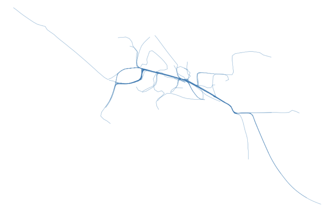
Above: An image rendering what these example traces look like for the sake of this exercise.

Note that these traces have been converted to EPSG 2163 - that is, they are in an equal area meter projection. The purpose is to have the line strings in a meter-based projection for the subsequent operations.

Cleaning

We will be describing these trace paths by the cells through which they pass. The cells I am referring to are the cells produced by gridding up the space within which these meter-projected trace segments exist. We will choose some level of resolution to work with (in the case of this post, 50 meters).

scale = 50  # meters

new_ls = []
for l in raw_linestrings:
    # creates points at intervals set by scale along the path
    # of the route and reconstructs the linestring associated
    n = int(l.length/scale)
    new_ls.append([l.interpolate(i * scale) for i in range(n + 1)])

We can iterate through the raw linestring traces (case as Shapely Linestrings) and interpolate along their paths so as to ensure there is data within each of the 50-meter cell grids that create a mesh over the area we are examining.

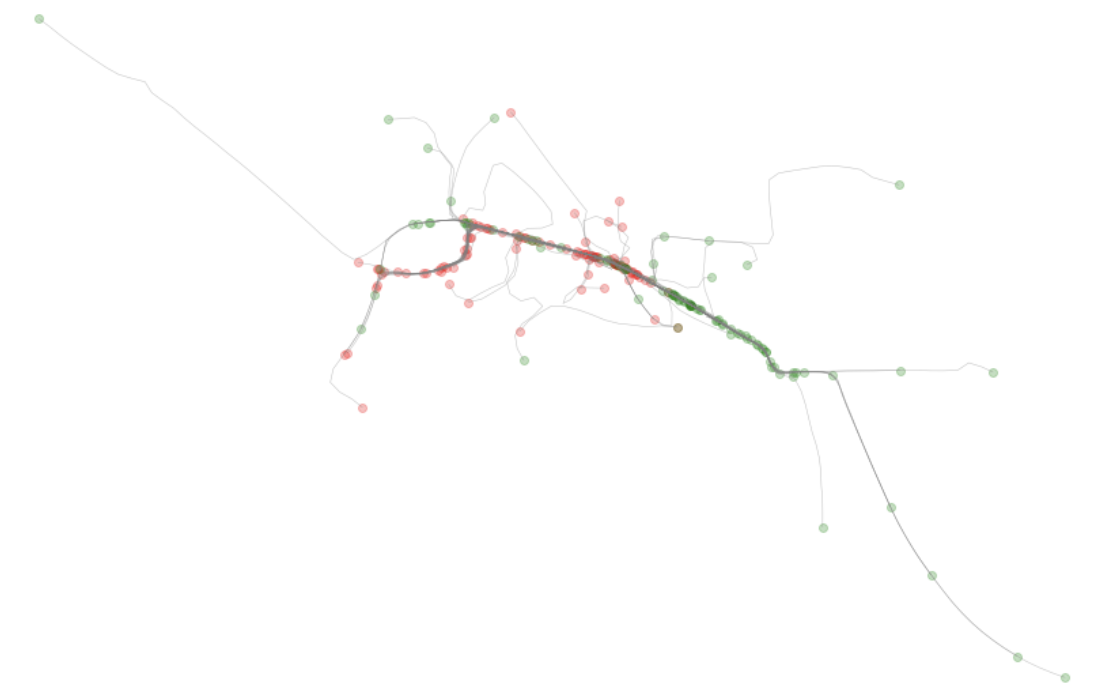
Above: We can see the results of the cleaned/processed data with start and end nodes highlighted.

Snapping to a grid

Now we can go through these traces and snap them to a grid. For each coordinate in the coordinate list that represents the LineString, snap that coordinate to the nearest cell grid node.

def _simple(c):
    scale = 50
    i = round(c / scale)
    return int(i * scale)

simplified_coords = []
for row in gdf.geometry:
    clean = []
    for cs in list(row.coords):
        newcs = [_simple(c) for c in cs]
        if len(clean) and (clean[-1] == newcs):
            # skip adding dupes
            continue
        clean.append(newcs)
        
    if len(clean) > 1:
        # do not add linesstrings if not enough coords
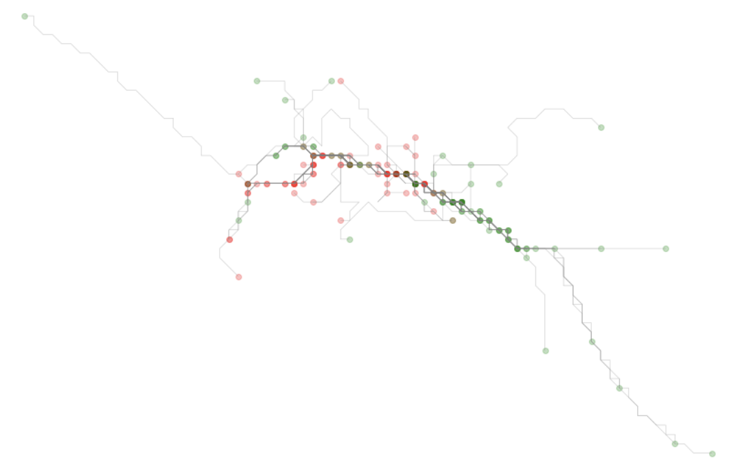
        simplified_coords.append(clean)

This will produced a simplified view of the traces, as shown below.

Identifying the target subarea

Now that we have a simplified version of each route, each traced route has common coordinates that act as hashes representing a specific cell - a cell id in essence. We can work through each aspect of that hash - representing the two dimensions along the x and the y axis - and get a frequency value for each.

# create 2 series that have frequencies of route segments for each column or row of axes
xd = {}
yd = {}
for sc in simplified_coords:
    for cs in sc:
        x = cs[0]
        if x not in xd:
            xd[x] = 0
        xd[x] += 1
        
        y = cs[1]
        if y not in yd:
            yd[y] = 0
        yd[y] += 1

xps = pd.Series(xd).sort_index()
yps = pd.Series(yd).sort_index()

We can then view these results as plots and observe how there are distributions that peak around a certain core along each axis.

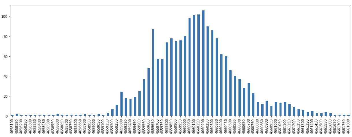
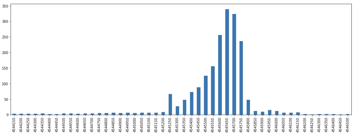
From these results we can subset to just the portion that represent the top, say, 90% of the observed frequencies for each axes.

# reduce the number of lines in consideration down to just those in this "hot zone"
keep_mask = []
for sc in simplified_coords:
    keep_mask.append(all(
        (x in xwantix and y in ywantix)
        for x, y in sc))

We can now subset to just this area and limit to the lines that solely have coordinate sets that fall entirely within this zone.

Scoring the lines

At this point, we have a target subset of trace lines. From these, we can go through each and look at each subsegment as a node-pair between two cells. We can take each of these edges and initialize them with count 0. As we iterate through each edge of each remaining trace, we can count up as we encounter an edge. This will allow us to get values for each subsegment and then represent each line as a sum of the values associated with each subsegment.

ctr = {}
keep_simple_lines = np.array(simplified_coords)[keep_mask]
for line in keep_simple_lines:
    for coord_pair in zip(line[:-1], line[1:]):
        cfr, cto = map(tuple, coord_pair)
        
        # initalize dict keys if not present
        if cfr not in ctr:
            ctr[cfr] = {}
        if cto not in ctr[cfr]:
            ctr[cfr][cto] = 0
            
        # increment as each is encountered
        ctr[cfr][cto] += 1

# now we can go back through and get the "total score" of each route
# and this can tell us which is the most common one
scores = []
for line in keep_simple_lines:
    sc = 0
    for coord_pair in zip(line[:-1], line[1:]):
        cfr, cto = map(tuple, coord_pair)
        sc += ctr[cfr][cto]
    scores.append(sc)

# here we can pick the busiest one from the pandas series
scoredf = pd.DataFrame({'scores': scores, 'lines': keep_simple_lines})

Getting the “core trunk”

At this point, extracting the line with the highest score is straightforward. We can take that line and plot it against all other lines.

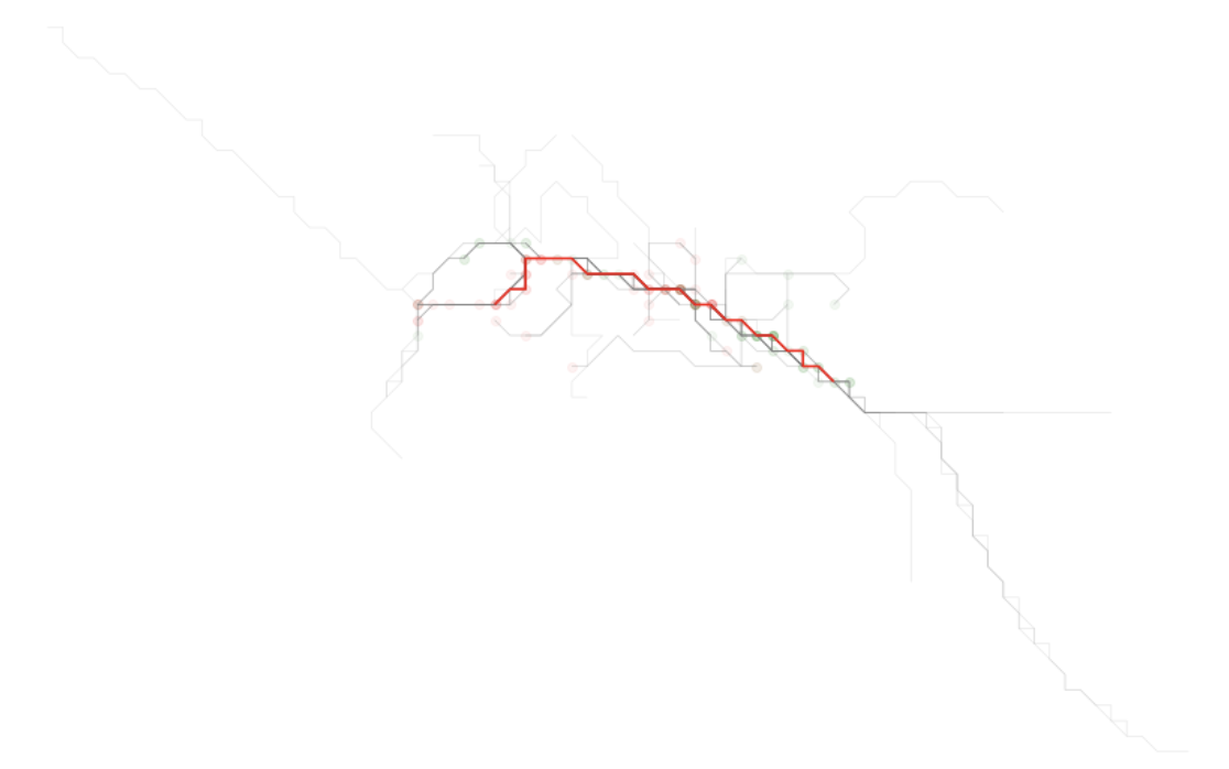
The result of this plot will show what was likely visually observable from the onset. But now we have highlighted the simplified form of the trace line that is busiest - that is, the one that represents a segment that is most traversed by the traces we were provided.

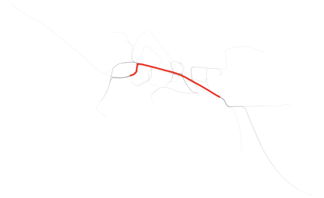
Just as we have the simplified shape, we also can go back and get that same trace in raw form and see how it is represented on the plot of the raw traces.

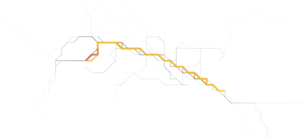
Finally, we can get the nth busiest and plot those as well as is shown above. The second and third lines happen to be quiet similar to the first, reinforcing that this corridor is most traversed.

At this point, we have extracted the busiest core trunk of all the trace routes provided. Next steps might be to find ways of extracting just the branches and then isolating only the most common branches.