Map matching over-simplified

Introduction

The purpose of this post is to demonstrate a crude but simple map matching algorithm that covers the basics of how a Hidden Markov Map Matching algorithm would work through a set of Python scripts that can be used to help illustrate the basic structure being employed in more advanced models.

In particular, this post attempts to “skip” the emission and transition probability models and replaces them with oversimplified algorithms to demonstrate roughly what they are intended to do, without actually getting into the specifics of each. Hopefully, this will clear the air to allow for the overall process to be more apparent. I should also note that a number of optimizations are foregone for the same reason - they simply make understanding the basic process more complicated (at least for me).

Network data

First, we need a road network represented as a graph. I’ll use OSMnx to query for OpenStreetMap data and hold it as a NetworkX MultiDiGraph. This is a directed graph that allows us to use shortest path (djikstra) functions to search for paths through the network with NetworkX “out of the box.”

For this example, I will use an area around downtown Oakland:

import osmnx as ox
from shapely.geometry import Polygon, box

p = Polygon([
            [
              -122.27465629577637,
              37.7983230783235
            ],
            [
              -122.26096630096434,
              37.7983230783235
            ],
            [
              -122.26096630096434,
              37.80761398306056
            ],
            [
              -122.27465629577637,
              37.80761398306056
            ],
            [
              -122.27465629577637,
              37.7983230783235
            ]
          ])

west, south, east, north = p.bounds
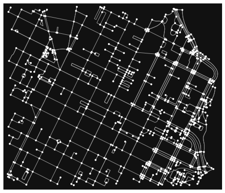
G1 = ox.graph_from_bbox(north, south, east, west)

We can plot the resulting graph. It should look like the following (the area near downtown Oakland, between it and the lake).

We also can convert this to a GeoDataFrame. This will come in handy for searching for edges and their attributes (though you could do this with the NetworkX graph object, too).

import geopandas as gpd

rows = []
for node_from, node_to, edge in G1.edges(data=True):
    if "geometry" in edge.keys():
        geometry = edge["geometry"]
    else:
        f = G1.nodes[node_from]
        t = G1.nodes[node_to]
        geometry = LineString([[f["x"], f["y"]], [t["x"], t["y"]]])
    base = {
        "from": node_from,
        "to": node_to,
        "id": edge["osmid"],
        "length": edge["length"],  # meters
        "geometry": geometry,
    }
    rows.append(base)

I’ll also hand create a set of breadcrumb trances to simulate a path that a map matcher would receive. I just drew a path around downtown Oakland:

from shapely.geometry import LineString

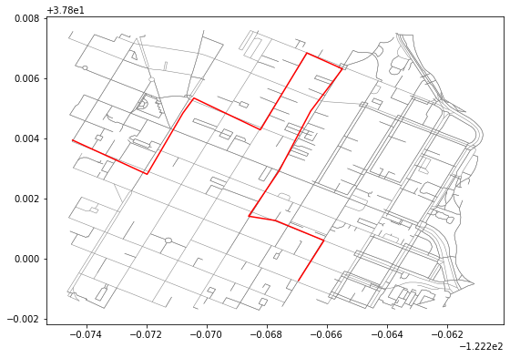
trace = LineString([[-122.26694762706754,37.79925985116652],[-122.26666867732999,37.79970068133491],[-122.2660920023918,37.800605646561564],[-122.26770132780074,37.80126899810456],[-122.26859986782071,37.80141311202907],[-122.26758331060408,37.80292417198254],[-122.26653456687926,37.804909907830265],[-122.26547777652739,37.806312818153785],[-122.26666331291199,37.80684261119228],[-122.26750552654266,37.80545242616099],[-122.26820826530457,37.80428685451822],[-122.27041840553284,37.80534222744762],[-122.27078318595886,37.80484209275872],[-122.27197408676149,37.8028076116559],[-122.27447390556335,37.80395201417224]])

We can plot the road network and the trace path together to see the path in red superimposed on the road network:

Helper methods

Let’s create a few helper methods before we continue to allow us to work with the data we were given. First, we will need to calculate the distance between coordinate points in some measure, such as meters. For that, I use the haversine formula:

from math import cos, sin, asin, sqrt, radians

def haversine(lat1, lon1, lat2, lon2):
    # convert decimal degrees to radians
    lon1, lat1, lon2, lat2 = map(radians, [lon1, lat1, lon2, lat2])
    # haversine formula
    dlon = lon2 - lon1
    dlat = lat2 - lat1
    a = sin(dlat / 2) ** 2 + cos(lat1) * cos(lat2) * sin(dlon / 2) ** 2
    c = 2 * asin(sqrt(a))
    km = 6371 * c
    return km * 1000

Similarly, I create a method to use the distance measure extract an edge given a breadcrumb coordinate trace point and create a reference object that tells me about the edge that is potentially paired with the trace point. Note that this is oversimplified and a number of optimizations could be made to improve how nearby edges get paired with a trance point, but this is intentionally simplified to communicate the overall methodology.

from shapely.geometry import Point

def get_edges(gdf, x, y, t=100):
    p = Point(x, y)
    
    near_edges = []
    for gdf_ix, row in gdf.iterrows():
        l = row["geometry"]
        p2 = l.interpolate(l.project(p))
        d = haversine(y, x, p2.y, p2.x)
        if d < t:
            near_edges.append({
                "id": gdf_ix,
                "distance": d,
                "from_node": row["from"],
                "to_node": row["to"],
            })
    return near_edges

Representing and tracking states in an HMM

Finally, we need to create a state node concept. What is this? You can imagine each breadcrumb in the telemetry trace I drew to be a state. That point is associated with the “real” path and represent the object being tracked being somewhere on the network at that point. So each breadcrumb represents a phase, or a state, on the network. We need to figure out two things:

1. What edge each state is associated with. There could be 2 or more nearby roads, which one was the object most likely on?
2. What edge the object then went to (it’s “transition”). Given that the object was likely on one road, what is the likelihood that it then went from there to some other road (edge)?

To do this, we each state to keep track of a few things associated with that trace breadcrumb:

1. The breadcrumb (or its index)
2. The associated edge it might be paired with

For the edge, we can keep track of some extra information to help us reference it later on:

1. How far away it (the trace point) is from that candidate edge
2. What is the start node for that road edge
3. What is the end node for that road edge

We also add in the concept of “terminal”. What this means is that there will be a start and an end, final state. We can imagine the states as columns side by side (see above illustration). The first column and the last only have one node each: they are “terminal”. We need to figure out the most likely edge for each state from that start node to the finish one.

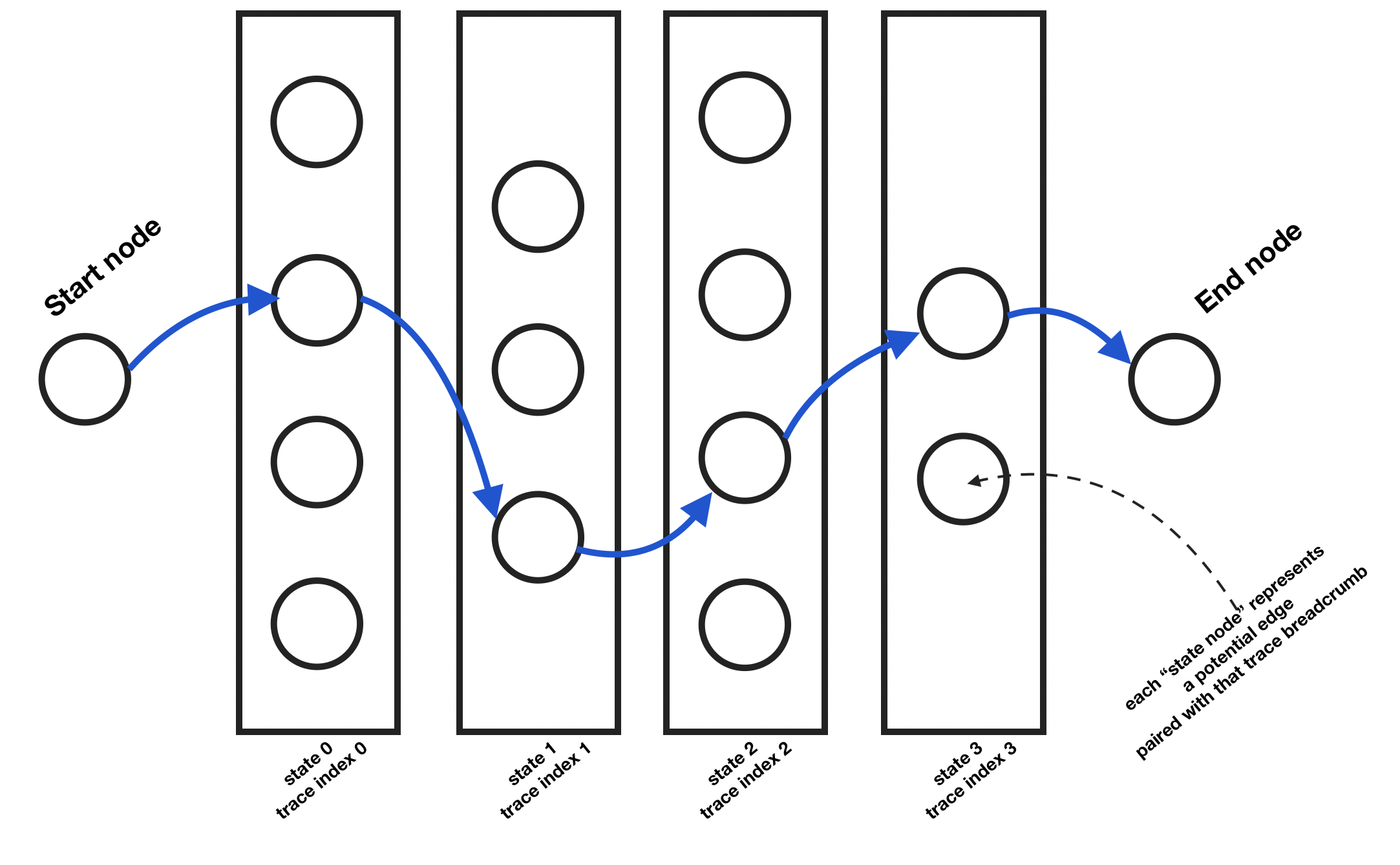
Each of those state nodes can be represented with the following class:

class StateNode():
    def __init__(self, trace_id, edge_id, distance, from_node, to_node, terminal=None):
        self.trace_id = trace_id
        self.edge_id = edge_id
        self.distance = distance
        self.from_node = from_node
        self.to_node = to_node
        self.terminal = terminal

Populating state columns with StateNodes

To initialize the state graph, we first need to iterate through each trace coordinate point and get the potential edges that are near it. Then, for each, we create a StateNode. Each of these get added to the graph and a link is created from each of the previous state column’s state nodes to each of the state

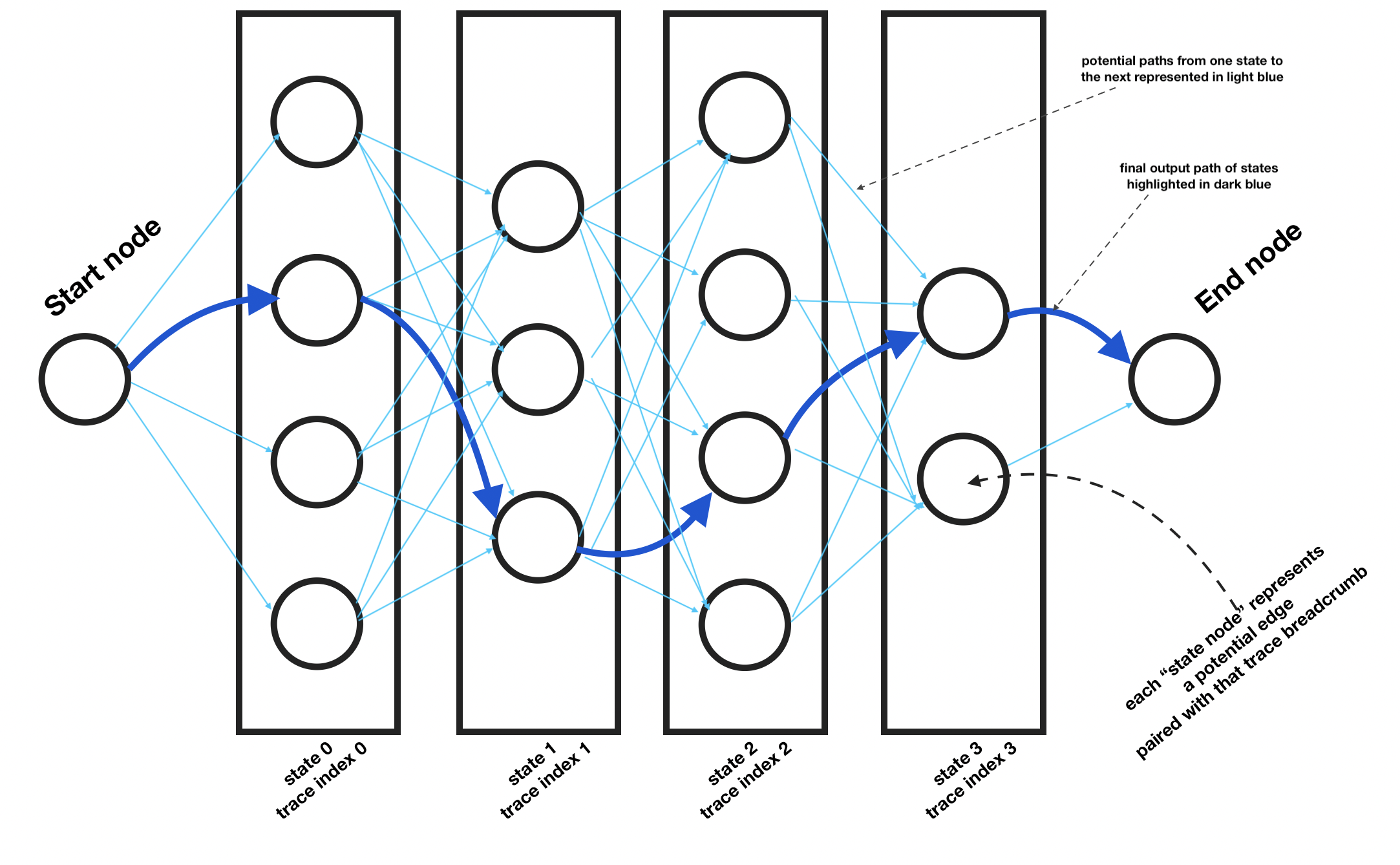
Once initialized as shown in the example chart above, we can see how each candidate state node in each state column is connected in one direction to each state node in the state column to the left. Then, on either end, are the start and end node.

Now, once this is created, we can search the “trellis” and find the path of least resistance from the start node to the end node in this state tree.

Here’s how I initialize the state tree and populate it with state nodes:

# initialize state graph
markov_chain = nx.DiGraph()

# initialize a start state with no real trace/edge associated
start_state_node = StateNode(None, None, None, None, None, "start")
markov_chain.add_node(start_state_node)

# initialize state layers to connect each
last_state = [start_state_node]

for trace_ix, xy in enumerate(trace.coords):
    current_state = []
    x, y = xy

    # Step 1: For each trace point get a list of edges
    edges = get_edges(gdf, x, y)

    # Step 2: Create adjacency list: each edge can tragnsition to every other edge
    for e in edges:
        next_state_node = StateNode(trace_ix, e["id"], e["distance"], e["from_node"], e["to_node"])
        
        markov_chain.add_node(next_state_node)
        current_state.append(next_state_node)
        
        for last_node in last_state:
            markov_chain.add_edge(last_node, next_state_node)
    
    # reset what last state is
    last_state = current_state
    
# add last state node placeholder
end_state_node = StateNode(None, None, None, None, None, "end")
markov_chain.add_node(end_state_node)
for last_node in last_state:
    markov_chain.add_edge(last_node, end_state_node)

Finding a path through the state tree

As mentioned earlier, we now need to traverse the state tree (from “left” to “right”). We want to create a methodology for evaluating each edge from one node to another in the state tree (not to be confused with the road network graph).

I’ve created this simplified get_edge_likelihood method to demonstrate how this would be done. It takes the start state node and the potential next state node and does 2 calculations:

1. First, it calculates the emission likelihood. This is the likelihood that the trace point is associated with the edge paired with it in this state node.
2. Second, I calculate the transmission likelihood. This is the likelihood of the path going from the preceding state’s edge to the next state node’s edge.

For both the emission and transition likelihood, far more complex functions are used in practice (and are often the subject of academic papers regarding improvements to HMM methods). For the purpose of this example, a very crude model will be proposed for each to simplify code and hopefully improve clarity.

For transition probability, we simply get the shortest path from one edge to another in the road graph and get the sum of those lengths. We then square that to exponentially penalize the longer routes.

Similarly, for emission probability, we take the Euclidean distance from the point to the nearest point on the paired edge. We then square that, as well, to exponentially penalize further edges.

Finally, we just add the two values together to create a weight score.

def get_edge_likelihood(start_node, end_node, attributes):
    # base conditions for terminal nodes
    if start_node.terminal == "start" or end_node.terminal == "end":
	# don't worry about first placeholder node to first "real" state node
	# and same for final placeholder terminal node
        return 1

    # calculate emission weight (likelihood of point being on this line)
    emission_weight = start_node.distance ** 2  # simplified to exponentially weight greater distances

    # calculate transition weight (likelihood of going from one edge to the next)
    try:
        graph_path = nx.dijkstra_path(G1, start_node.to_node, end_node.from_node, weight="length")
        lengths = []
        for eid_from, eid_to in zip(graph_path[:-1], graph_path[1:]):
            lengths.append(G1[eid_from][eid_to][0]["length"])
        distance = sum(lengths)
    except nx.NetworkXNoPath:
        # fallback for impossible paths
        distance = 1_000_000
    
    transition_weight = distance ** 2  # simplified to exponentially weight greater distances

    # simplified example of combining the two factors
    return emission_weight + transition_weight

We can use this function to calculate the path of least resistance (lower weight paths) from the start node to the end node.

calculated_path = nx.dijkstra_path(markov_chain, start_state_node, end_state_node, weight=get_edge_likelihood)

Constructing the full map matched path

We can visualize the resulting calculated_path result by finding the paired nodes with the final set of state nodes that calculated_path is comprised of. For each state node pair, get the path between the two edges if they are not connected. After that, get the geometries for the list of edge ids and create an array of LineString geometries. We can then plot that and view the paired result (blue) against the raw (red) and the road network (grey).

# plot the base map in grey
ax = gdf.plot(figsize=(9,9), lw=0.5, color="grey")

# raw trace in red
gpd.GeoSeries([trace]).plot(ax=ax, color="red")

# map-matched trace in blue
calculated_path_trimmed = [c for c in calculated_path if c.edge_id is not None]

path_edges = []
for cp in calculated_path_trimmed:
    row = gdf.loc[cp.edge_id]

    if len(path_edges) == 0:
        path_edges.append(row)
        continue
    
    last_edge = path_edges[-1]
    if last_edge.to == row["from"]:
        path_edges.append(row)
        continue
    
    intermediate_path = nx.dijkstra_path(G1, last_edge.to, row["from"], weight="length")
    for ip_id_from, ip_id_to in zip(intermediate_path[:-1], intermediate_path[1:]):
        mask_1 = gdf["from"] == ip_id_from
        mask_2 = gdf["to"] == ip_id_to
        ip_row = gdf[mask_1 & mask_2].head(1).squeeze()
        path_edges.append(ip_row)


gpd.GeoSeries([row["geometry"] for row in path_edges]).plot(ax=ax, color="blue")

This will generate the following result image:

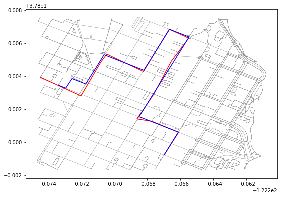
Discussing results

If you look at the left side of the resulting plot, you can see that the map matched path differs from the raw path and takes a different route (going north instead of south around a block).

This is an issue with the get_edge_likelihood function and is a nice segue into all the optimization work done with map matching with HMM that improves how transmission and emission likelihood values are calculated which, in turn, adjusts the weights that are calculated between state nodes and thus resulting state paths.

Also, there are a number of optimizations also possible during the state tree creation, to further limit the number of state nodes that are created. This improves the runtime of the map matching algorithm by using heuristics to toss potential edges that are in all likelihood unreasonable candidates.