RAPTOR transit routing algorithm basics

Introduction

RAPTOR stands for: “novel RoundbAsed Public Transit Optimized Router.” It’s based on this paper by Microsoft Research and demonstrates a simple method for traversing published transit schedules to determine what the optimal path is between two stops.

There are numerous optimizations presented both in this paper and in broader discussion of the algorithm. The goal of this post is to skip all of that discussion and show the most stripped down version of the algorithm possible, to clearly demonstrate it’s fundamental concept. This version is not intended to be performant, but it does work and is hopefully simple enough to be easily digestible.

I’ve included all this work in a Github Gist notebook for reference as well. In this post, I will take snippets from that code, but you can reference the original for the total set of scripts to run end-to-end. In the future, I’ll follow up on this post with an example that also brings in some of the additional performance optimizations presented.

Base data and tools

For this example, we will be using AC Transit’s latest GTFS feed. I pulled this down on September 8, 2020. The data was pulled from their data resource center. I’ll be using a few key libraries in python.

First, I will use partridge to parse the raw GTFS and load it up as pandas data frames. I will also use Geopandas to perform some geo-based operations to compute proximities with nearby stops for the purpose of adding in transfers between lines as footpath (or, walk) transfers.

Algorithm

The RAPTOR algorithm has 3 main steps. Note I will be using terminology based on GTFS to describe components of the transit feed.

Get all stops currently accessible (initially, just the starting origin stop) and find associated trip ids.
For all stops in associated with each trip id, use arrival and departure data to figure out how long to reach each other stop in the trip.
For each reachable stop, see if there are other stops nearby that can be walked to (footpath transfers).

raptor_algo_diagram

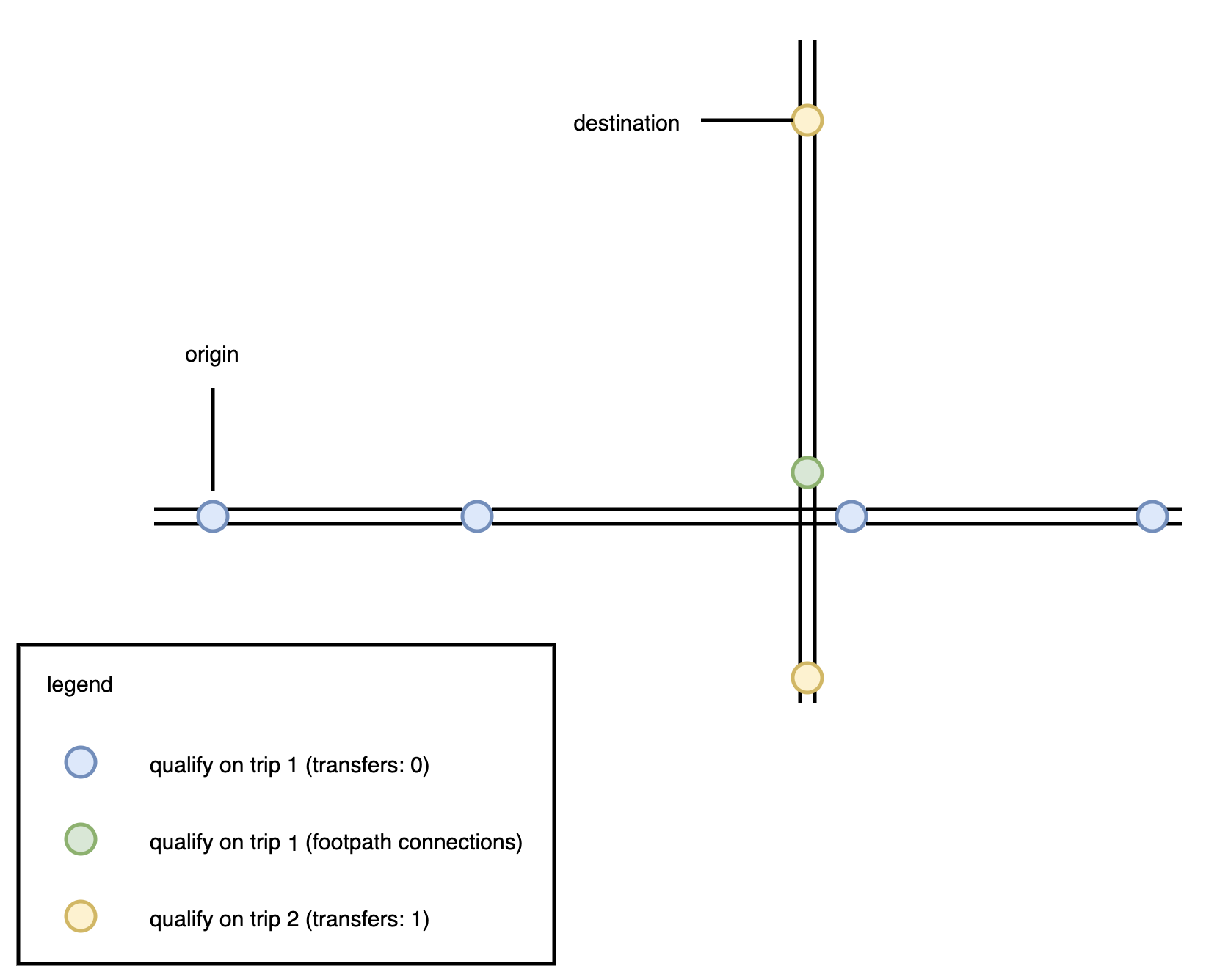
We can visualize this with the above graphic. First, we can reach everything along the trips along the stop that we start at. This is just the east-west route at first. Then we can find nearby transfers (the green dot) and add these to our qualifying stop ids. On the next iteration (a trip with 1 transfer), we now can consider all possibilities from all the stops from the first iteration: the blue and the green stops. This opens up all the trips that serve the yellow stops now, which lets us navigate to the destination stop node.

Loading in the data

First let’s read in the GTFS data. We’ll just work with the busiest day for this example.

import partridge as ptg

# load a GTFS of AC Transit
path = 'gtfs.zip'
_date, service_ids = ptg.read_busiest_date(path)
view = {'trips.txt': {'service_id': service_ids}}
feed = ptg.load_feed(path, view)

Next, we will also want to convert the stops to shapes so we can find nearest stops.

import geopandas as gpd
import pyproj
from shapely.geometry import Point

# convert all known stops in the schedule to shapes in a GeoDataFrame
gdf = gpd.GeoDataFrame(
    {"stop_id": feed.stops.stop_id.tolist()},
    geometry=[
        Point(lon, lat)
        for lat, lon in zip(
            feed.stops.stop_lat,
            feed.stops.stop_lon)])
gdf = gdf.set_index("stop_id")
gdf.crs = {'init': 'epsg:4326'}

# re-cast to meter-based projection to allow for distance calculations
aeqd = pyproj.Proj(
    proj='aeqd',
    ellps='WGS84',
    datum='WGS84',
    lat_0=gdf.iloc[0].geometry.centroid.y,
    lon_0=gdf.iloc[0].geometry.centroid.x).srs
gdf = gdf.to_crs(crs=aeqd)

Finally, we want to get the start and end node for our example.

# let's use this example origin and destination
# to find the time it would take to go from one to another
from_stop_name = "Santa Clara Av & Mozart St"
to_stop_name = "10th Avenue SB"

# QA: we know the best way to connect these two is the 51A -> 1T
# if we depart at 8:30 AM, schedule should suggest:
#     take 51A 8:37 - 8:49
#     make walk connection
#     take 1T 8:56 - 9:03
# total travel time: 26 minutes

# look at all trips from that stop that are after the depart time
departure_secs = 8.5 * 60 * 60

# get all information, including the stop ids, for the start and end nodes
from_stop = feed.stops[feed.stops.stop_name == from_stop_name].head(1).squeeze()
to_stop = feed.stops[["10th Avenue" in f for f in feed.stops.stop_name]].head(1).squeeze()

# extract just the stop ids
from_stop_id = from_stop.stop_id
to_stop_id = to_stop.stop_id

Helper methods

There will be 3 main helper methods to help with each of the main steps that were stated above. First, we need to get the associated trips for a given stop.

def get_trip_ids_for_stop(feed, stop_id: str, departure_time: int):
    """Takes a stop and departure time and get associated trip ids."""
    mask_1 = feed.stop_times.stop_id == stop_id
    mask_2 = feed.stop_times.departure_time >= departure_time

    # extract the list of qualifying trip ids
    potential_trips = feed.stop_times[mask_1 & mask_2].trip_id.unique().tolist()
    return potential_trips

Now, given those trips, we can iterate through the stops that we can reach so far and find all other stops we can reach from these identified trips. Then, we can compute the time it takes to reach those stops and if it is faster than what we currently have (or we do not yet have them as reachable), we can add them to our managing object that holds all accessible stops.

def stop_times_for_kth_trip(
    from_stop_id: str,
    stop_ids: List[str],
    time_to_stops_orig: Dict[str, Any],
) -> Dict[str, Any]:
    # prevent upstream mutation of dictionary
    time_to_stops = copy(time_to_stops_orig)
    stop_ids = list(stop_ids)

    for i, ref_stop_id in enumerate(stop_ids):
        # how long it took to get to the stop so far (0 for start node)
        baseline_cost = time_to_stops[ref_stop_id]

        # get list of all trips associated with this stop
        potential_trips = get_trip_ids_for_stop(feed, ref_stop_id, departure_secs)
        for potential_trip in potential_trips:

            # get all the stop time arrivals for that trip
            stop_times_sub = feed.stop_times[feed.stop_times.trip_id == potential_trip]
            stop_times_sub = stop_times_sub.sort_values(by="stop_sequence")

            # get the "hop on" point
            from_her_subset = stop_times_sub[stop_times_sub.stop_id == ref_stop_id]
            from_here = from_her_subset.head(1).squeeze()

            # get all following stops
            stop_times_after_mask = stop_times_sub.stop_sequence >= from_here.stop_sequence
            stop_times_after = stop_times_sub[stop_times_after_mask]

            # for all following stops, calculate time to reach
            arrivals_zip = zip(stop_times_after.arrival_time, stop_times_after.stop_id)
            for arrive_time, arrive_stop_id in arrivals_zip:
                
                # time to reach is diff from start time to arrival (plus any baseline cost)
                arrive_time_adjusted = arrive_time - departure_secs + baseline_cost

                # only update if does not exist yet or is faster
                if arrive_stop_id in time_to_stops:
                    if time_to_stops[arrive_stop_id] > arrive_time_adjusted:
                        time_to_stops[arrive_stop_id] = arrive_time_adjusted
                else:
                    time_to_stops[arrive_stop_id] = arrive_time_adjusted

    return time_to_stops

For the 3rd step, we can calculate potential transfers. These are nearby stops that we assume you can walk to. We will use the GeoDataFrame to just find nearby stops to each qualifying stop. Of course, this is very inefficient, but we are keeping it simple for the purpose of demonstrating the basics of this algorithm.

# assume all xfers are 3 minutes
TRANSFER_COST = (5 * 60)

def add_footpath_transfers(
    stop_ids: List[str],
    time_to_stops_orig: Dict[str, Any],
    stops_gdf: gpd.GeoDataFrame,
    transfer_cost=TRANSFER_COST,
) -> Dict[str, Any]:
    # prevent upstream mutation of dictionary
    time_to_stops = copy(time_to_stops_orig)
    stop_ids = list(stop_ids)

    # add in transfers to nearby stops
    for stop_id in stop_ids:
        stop_pt = stops_gdf.loc[stop_id].geometry

        # TODO: parameterize? transfer within .2 miles
        meters_in_miles = 1610
        qual_area = stop_pt.buffer(meters_in_miles/5)
        
        # get all stops within a short walk of target stop
        mask = stops_gdf.intersects(qual_area)

        # time to reach new nearby stops is the transfer cost plus arrival at last stop
        arrive_time_adjusted = time_to_stops[stop_id] + TRANSFER_COST

        # only update if currently inaccessible or faster than currrent option
        for arrive_stop_id, row in stops_gdf[mask].iterrows():
            if arrive_stop_id in time_to_stops:
                if time_to_stops[arrive_stop_id] > arrive_time_adjusted:
                    time_to_stops[arrive_stop_id] = arrive_time_adjusted
            else:
                time_to_stops[arrive_stop_id] = arrive_time_adjusted
    
    return time_to_stops

Bringing it all together

Now that we have the 3 helper functions, we can run them together to generate an iterator that iterates through the number of transfers we have set as a limit and keeps finding or updating how long it takes to reach all/any stops in the system. At the end of the iterations, we see if our destination stop is there and we get a resulting timeframe for reaching it.

Note again that there is plenty of optimizations to be introduced but, again, the purpose is to just show the fundamental concept of the algorithm.

import time

# initialize lookup with start node taking 0 seconds to reach
time_to_stops = {from_stop_id: 0}

# setting transfer limit at 1
TRANSFER_LIMIT = 1
for k in range(TRANSFER_LIMIT + 1):
    logger.info("\nAnalyzing possibilities with {} transfers".format(k))
    
    # generate current list of stop ids under consideration
    stop_ids = list(time_to_stops.keys())
    logger.info("\tinital qualifying stop ids count: {}".format(len(stop_ids)))
    
    # update time to stops calculated based on stops accessible
    tic = time.perf_counter()
    time_to_stops = stop_times_for_kth_trip(from_stop_id, stop_ids, time_to_stops)
    toc = time.perf_counter()
    logger.info("\tstop times calculated in {:0.4f} seconds".format(toc - tic))

    added_keys_count = len((time_to_stops.keys())) - len(stop_ids)
    logger.info("\t\t{} stop ids added".format(added_keys_count))
    
    # now add footpath transfers and update
    tic = time.perf_counter()
    stop_ids = list(time_to_stops.keys())
    time_to_stops = add_footpath_transfers(stop_ids, time_to_stops, gdf)
    toc = time.perf_counter()
    logger.info("\tfootpath transfers calculated in {:0.4f} seconds".format(toc - tic))

    added_keys_count = len((time_to_stops.keys())) - len(stop_ids)
    logger.info("\t\t{} stop ids added".format(added_keys_count))
    
assert to_stop_id in time_to_stops, "Unable to find route to destination within transfer limit"
logger.info("Time to destination: {} minutes".format(time_to_stops[to_stop_id]/60))

Here is the logged output from the above run with AC Transit data and start and end nodes set up earlier. The resulting time is 35.5 minutes which is the same as what you would get in a service like Google Maps (estimated 36 minutes).

Analyzing possibilities with 0 transfers
    inital qualifying stop ids count: 1
    stop times calculated in 0.8255 seconds
        28 stop ids added
    footpath transfers calculated in 0.6502 seconds
        103 stop ids added

Analyzing possibilities with 1 transfers
    inital qualifying stop ids count: 132
    stop times calculated in 137.7573 seconds
        828 stop ids added
    footpath transfers calculated in 20.8401 seconds
        1053 stop ids added
Time to destination: 35.5 minutes

Conclusion

I hope this was helpful in demonstrating with code the basic concept of the RAPTOR transit routing algorithm presented in this paper. This is just a skeleton. It would be easy to introduce some of the optimizations discussed in the paper as well as modify how trips and stop paths are tracked to daylight more information other than just time to reach a stop (such as the path, the associated routes, and the number of transfers).