Handling Noisy Probes and Unrealistic Paths
This is a follow up to my last post; discussing issues I saw when map matching and some notes on improving against those problems. One issue that became increasingly obvious after running the matcher against real probe data is how noisy probes interact with dense road networks.
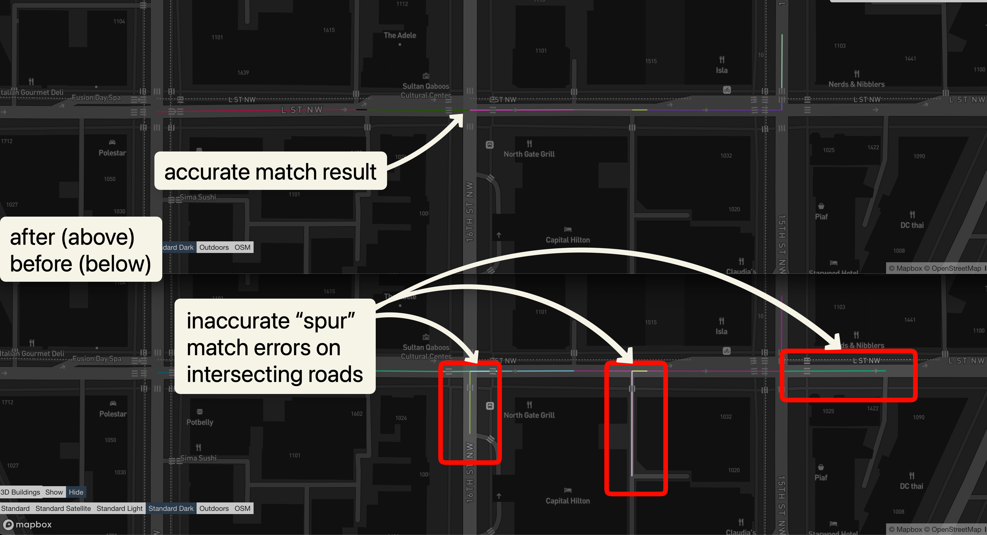
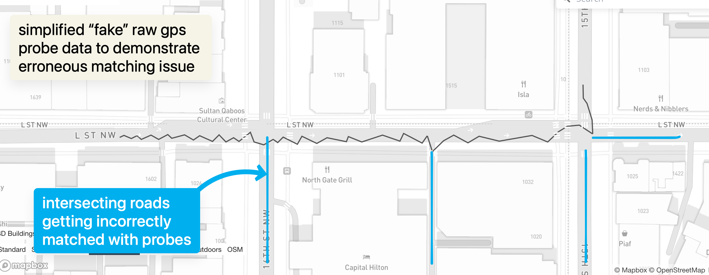
In urban environments especially (as shown in above example), a single probe can be spatially close to multiple candidate ways: a main road, a frontage road, a service alley, or even a perpendicular side street. When the scoring model is too permissive, the matcher will occasionally “snap” to one of these intersecting roads even though the vehicle never really traveled down it.
Context: From Naive Viterbi to Practical Heuristics
None of the strategies described below are novel. In fact, they’re fairly standard ideas in map matching and routing systems more broadly.
In my previous post, Lightweight HMM Map Matching in Go, I intentionally started from a very naive place: a straightforward Viterbi implementation over candidate road segments, with minimal transition logic and few guardrails. That was useful as a baseline, but it also made the failure modes extremely obvious once real probe data entered the picture.
This follow-up is really about identifying the minimum set of logical checks needed to make the matcher behave plausibly, without turning it into a heavy, compute-intensive routing engine. The goal isn’t to perfectly model driver behavior or handle every edge case — it’s to avoid the most common and most egregious matching errors while preserving simplicity, performance, and operational clarity.
Everything that follows can be thought of as adding just enough structure around the HMM to constrain it to realistic paths, rather than letting it “mathematically” solve the problem in ways that no real vehicle ever would.
The Problem: Intersections + Noise = Bad Matches
When this happens, the downstream effect is worse than just a single bad segment. The HMM will often try to recover by immediately transitioning back to the original road. The resulting matched path looks something like:
-
main road
-
sudden turn onto a side street, go down to next intersection
-
immediate u-turn (no matter how unrealistic)
-
back onto the main road (could have just proceeded straight)
From a routing perspective, this is clearly unrealistic. From a scoring perspective, however, the original model didn’t strongly discourage this behavior. Short segments, small distances, and weak penalties made these transitions look acceptable.
Over longer traces, these errors compound into paths that zig-zag through intersections in ways no real vehicle would.
First Fix: Penalize U-Turns
The most obvious initial fix was to explicitly penalize u-turns.
If a transition implies a near-180° change in heading between consecutive matched ways, that transition should be costly. In real driving, u-turns are rare, deliberate, and usually constrained to specific locations. They should not be the default recovery mechanism for noisy probes.
Adding a u-turn penalty immediately reduced the most egregious back-and-forth behavior.
But once that was in place, a broader issue became clear.
Generalizing the Idea: Penalize Turns, Not Just U-Turns
U-turns are just the extreme case. In practice, many bad matches involve sharp turns that aren’t full reversals but are still implausible given the trace.
This led to a more general approach: add a turn cost based on heading change.
Instead of a binary “u-turn or not” check, transitions are penalized proportionally to how sharp the turn is. Small heading changes are cheap. Large heading changes get increasingly expensive.
This makes the matcher prefer smooth, continuous motion unless the probes strongly indicate otherwise.
Road Class Matters
Even with turn penalties, another pattern showed up repeatedly: many of the accidental detours were happening on low-class roads.
Alleys, service roads, and tiny access lanes are often geometrically close to major roads. A single noisy probe can easily fall closer to an alley than to the primary road the vehicle is actually on.
What made these cases especially bad was the sequence:
-
primary road → alley
-
short travel
-
u-turn
-
back to primary road
From a modeling standpoint, this should be extremely unlikely.
To address this, transition costs now also consider road class. Transitions from higher-class roads (e.g. primary or secondary roads) to much lower-class roads (e.g. alleys or service roads) are penalized heavily, especially when followed by sharp turns or u-turns.
This reflects real behavior: drivers don’t casually dip into alleys and immediately reverse course unless they are intentionally accessing something there.
Distance and Probe Coverage
Another important signal is how much evidence there is that a candidate way was actually traveled.
If a candidate road is only supported by a single probe, especially when neighboring probes align well with another road, the matcher should be skeptical. A single noisy observation should not be enough to justify a detour.
To capture this, transition scoring now incorporates:
-
Distance traveled on the candidate way
-
Probe coverage: how well the trace aligns with the geometry over multiple points
Short, weakly supported segments get penalized relative to longer, well covered ones. This makes it much harder for the matcher to justify hopping onto a side road for just one probe.
Cleanup Pass: Fixing What Still Slips Through
Even with improved scoring, some unrealistic paths can still sneak through—especially in dense downtown grids or highly noisy traces.
To address this, I added a lightweight cleanup step that runs after the main matching pass. This step walks back through the matched result and looks for obvious anomalies:
-
extremely short detours
-
rapid back-and-forth transitions
-
isolated low-class road segments sandwiched between higher class roads
When detected, these segments can be collapsed or replaced with more plausible alternatives from the surrounding context.
This cleanup isn’t meant to “fix everything,” but it acts as a final sanity check to smooth out pathological cases that the probabilistic model occasionally produces.
Performance Impact of the Added Heuristics
After adding these heuristics, I re-ran the exact same benchmark harness used in the previous post to sanity-check whether match quality improvements came with a performance cost.
Updated Results
Total routes:   10000
Successful:     10000 (100%)
Total time:     19.82s
Throughput:     ~504.6 routes/sec

Median latency: ~136ms
P95 latency:    ~321ms
P99 latency:    ~392ms
Compare this to the old results from the last blog post:
Total routes:   10000
Successful:     10000 (100%)
Total time:     34.29s
Throughput:     ~291.6 routes/sec

Median latency: ~294ms
P95 latency:    ~913ms
P99 latency:    ~980ms
Observations
At face value, the updated matcher is noticeably faster and has significantly better tail latencies. That said, I want to be careful not to over-interpret this result.
These changes were primarily about constraining the state space — discouraging implausible transitions early rather than allowing them and “fixing” them later. It’s entirely possible that the improved performance is partially due to the Viterbi pass having fewer viable transitions to consider, rather than any intentional optimization.
It’s also possible some of this improvement is simply noise or an artifact of how the benchmark exercises the matcher. Either way, the important takeaway is not that the matcher got faster, but that it did not get meaningfully slower.
Given that these heuristics are lightweight (simple arithmetic, heading comparisons, and metadata checks), they appear to improve match quality without introducing noticeable computational overhead. For the intended use case — high-volume, short traces — that’s exactly the tradeoff I was hoping for.
Final thoughts
None of these changes are particularly complex on their own. The improvement comes from stacking multiple weak signals:
-
turn cost
-
u-turn penalties
-
road class awareness
-
distance and coverage weighting
-
post-processing cleanup
All these need to work together to produce reliable results. These are all heuristics in the end - need to also understand the quality of the input data. Helps to know what the input data looks like - if it fits a common pattern, then we are better suited to optimize for that versus a more general purpose use case.