Context
One of the more common failure modes in real-time geospatial systems has nothing to do with algorithms being wrong. It’s that the real world refuses to stay still.
This post walks through a practical pattern for handling high-volume, real-time location data where part of your pipeline is explicitly geo-constrained (map matching, spatial joins, routing lookups, etc.), while the rest of the system is not. We’ll look at why static geographic partitioning breaks down, and how to use real-time monitoring plus fast redeploys to continuously rebalance work instead of over-allocating forever.
The canonical pipeline shape
Most real-time geo pipelines look roughly like this:
┌─────────────────┐         ┌──────────────────────┐         ┌─────────────────┐
│   Aspatial      │         │  Geo-Constrained     │         │   Downstream    │
│  Data Stream    │────────>│    Transformer       │────────>│    Consumers    │
│ (ex: Kinesis)   │         │                      │         │                 │
└─────────────────┘         └──────────────────────┘         └─────────────────┘
-
You ingest a jumbled, global stream of location events.
-
You pass it through a geo-constrained transformer (map matching is a common example).
-
After enrichment, the data fans out to downstream consumers that generally don’t care about geography anymore.
The critical detail is that only one section of the pipeline has strict geographic constraints. That section is where everything gets interesting — and unstable.
Why geo-partitioning is inherently unstable
The issue isn’t poor engineering; it’s that real-world spatial data is non-stationary.
Volume changes come from:
-
Day/night cycles
-
Commute peaks
-
Weather
-
Local events
-
Virality and feedback loops
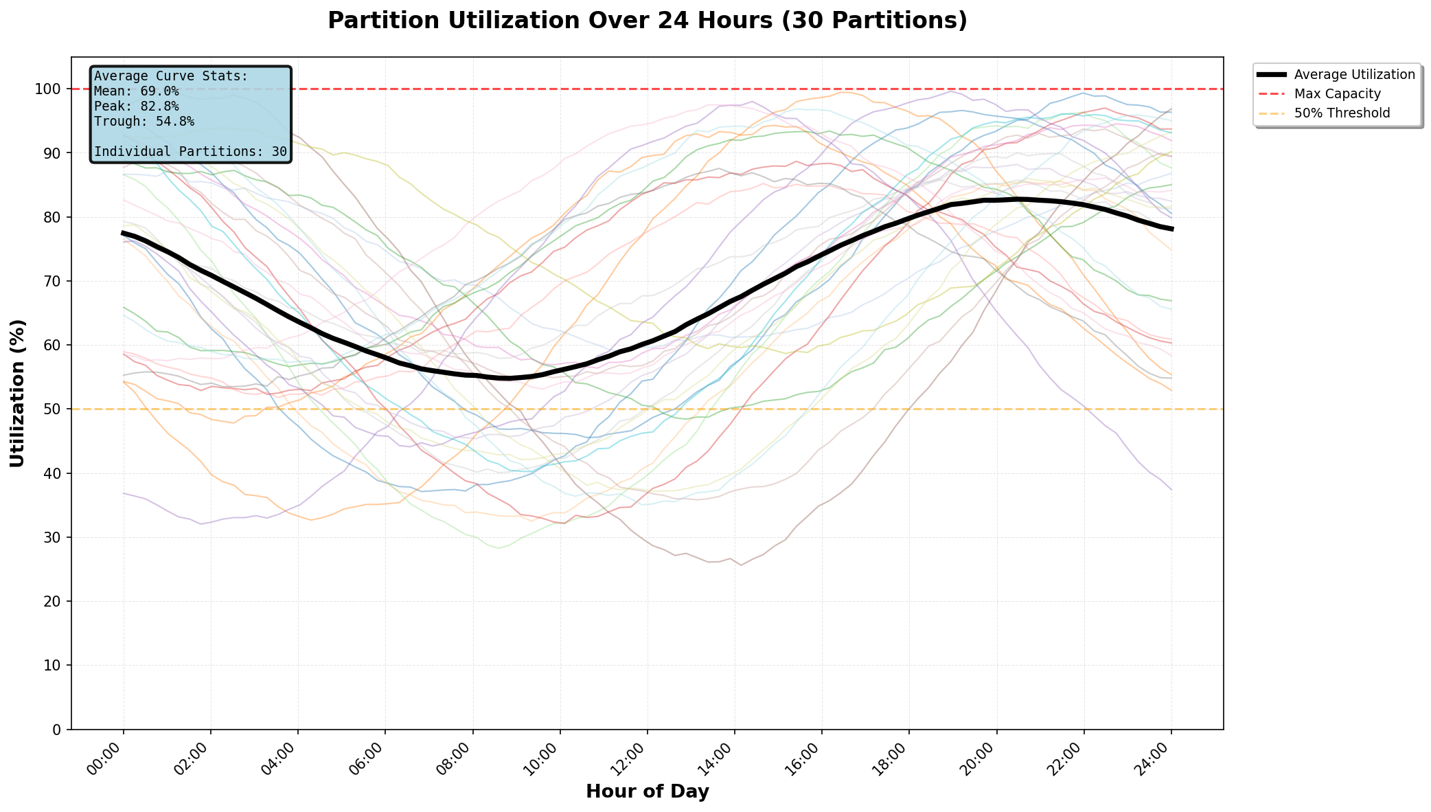
Above image is a generic example showing how even with the best partitioning strategy, various partitions are subject to time-of-day resource demand fluctuations.
Even if global throughput is stable, regional load never is. One city lights up while another goes quiet. Then they swap.
A common mitigation is “smart” partitioning:
-
Pair cities on opposite sides of the globe
-
Mix antipodal time zones (Johannesburg + Honolulu, etc.)
-
Try to smooth diurnal cycles statistically
This helps — but it never solves the problem. You still end up with:
-
Hot partitions you must size for worst-case load
-
Cold partitions wasting compute most of the day
-
A few megacities that remain pathological outliers no matter how clever your scheme is
At scale, this means systematic over-allocation.
Real goal: rebalance, don’t predict
Instead of trying to design the perfect static partitioning algorithm, the goal shifts: Continuously rebalance the geo-constrained service based on observed load.
That means:
-
Monitoring real-time spatial volume
-
Recomputing partitions from current conditions
-
Redeploying the geo-service frequently enough to track reality
This post assumes a few important properties:
-
Fast startup: New partition workers can come online in seconds to minutes.
-
Blue-green deploys: You can stand up a new geo-partitioned service in parallel and flip traffic.
-
No instantaneous spikes: Because this is real-world geo data, even “viral” events ramp over minutes (at least, if not longer), and definitely not less (not milliseconds).
Under those assumptions, dynamic rebalancing becomes not only possible, but practical.
A miniaturized example
To make this concrete, we’ll shrink the problem down to a single metro area instead of the globe. We define:
-
Two system states: before and after
-
The “after” state has:
- ~2× the total points - and thus higher overall activity
- More hotspots of dense activity vs. the prior state
Each partition is capped at 2,500 points. The goal is to build contiguous geographic partitions that get as close to that limit as possible.
State 1: before
Here’s a representative partitioning outcome:
Total partitions: 12
Max points per partition: 2500

Partition   0:   2272 points (90.9%)
Partition   1:   2265 points (90.6%)
Partition   2:   2257 points (90.3%)
Partition   3:   2254 points (90.2%)
Partition   4:    396 points (15.8%)
Partition   5:    371 points (14.8%)
Partition   6–11: < 200 points each
A few things jump out: First; hot areas pack efficiently. Secondly, cold regions fragment into many tiny partitions that are not contiguous. These tail partitions can safely be merged later. So far, so good.
State 2: naive preservation breaks down
Now activity doubles and new hotspots appear. If we try to preserve existing partitions and only split the ones that overflow, we get something like this:
Partition   0: 3243 points (129.7%)
Partition   2: 3689 points (147.6%)
...
Total partitions: 21
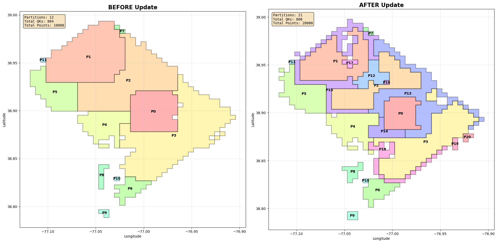
We’ve avoided redoing everything, but introduced a new problem:
-
Weird “edge” partitions appear
-
Shapes shrink inward awkwardly
-
Utilization becomes noisy and uneven
These liminal partitions are artifacts of trying to respect history that no longer matters.
Resolution: rebuild from scratch
If your deploys are fast, there’s no reason to preserve old partitions at all. Instead:
-
Ignore the previous state
-
Repack all quadkeys based on current load
-
Blue-green swap the new configuration in
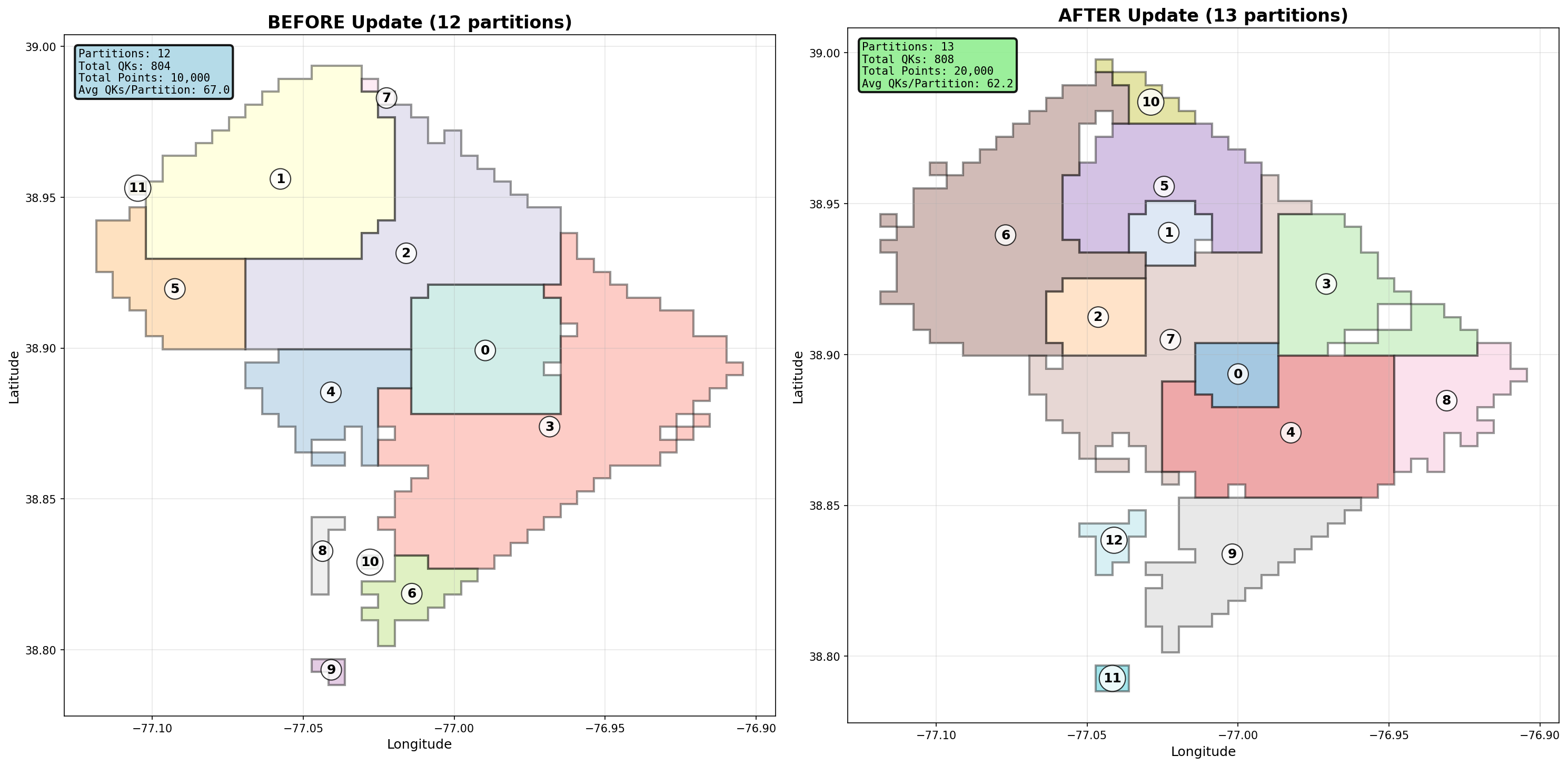
The result is cleaner, fewer partitions, and higher average utilization:
Total partitions: 13
Mean utilization: 61.5%
Median utilization: 90.1%
Cold tail partitions still exist, but they’re smaller in number, they’re easy to group together, they don’t pollute the hot path. This turns partitioning into a stateless optimization problem, not a migration problem.
Why this matters: allocation mismatch
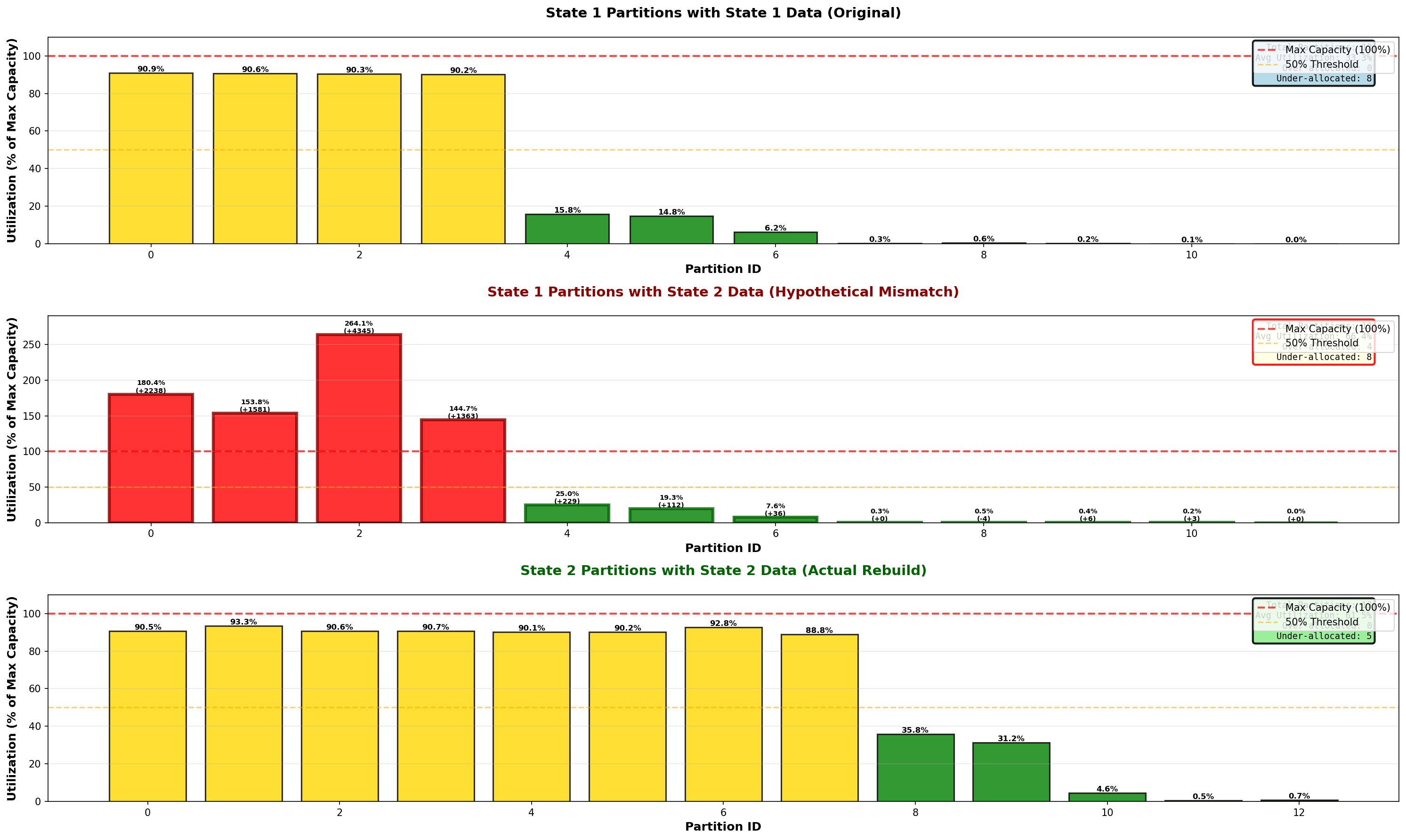
To see the cost of not rebalancing, apply State-2 data to State-1 partitions:
Partition 2: 2257 → 6602 points (264% utilized)
Partition 0: 2272 → 4510 points (180% utilized)
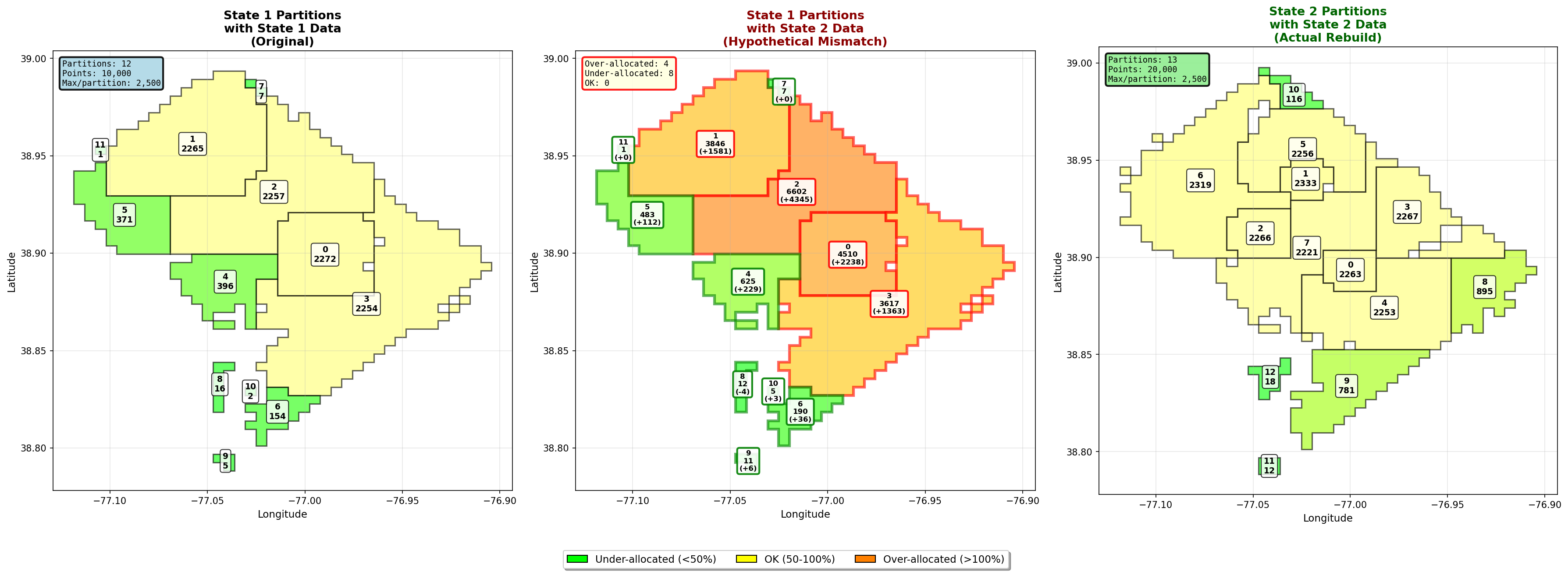
You’d need to provision 2–3x the resources just to survive peak load in a single partition — and every other partition would sit idle most of the time. Dynamic rebalancing converts that worst-case sizing problem into a steady-state one.
System architecture
At a high level, the control plane for this looks like:
Kinesis Stream

   → Managed Flink (Kinesis Data Analytics / EKS)
       - Job Manager
       - Task Managers
       - State backend (S3)
       - Checkpoints (S3)

   → DynamoDB / S3
Managed Flink on AWS makes this pattern pretty easy to implement. You get a continuously running, stateful streaming job without having to own the cluster lifecycle, and can still retain enough control to make dynamic reconfiguration viable.
Flink’s execution model lines up well with what is needed:
-
It has native keyed aggregation: Counting by quadkey is a first-class operation (
keyBy → window / process) -
Continuous output: do not need to wait for batch windows to close. Emit rolling aggregates on a cadence (e.g. every 30–60 seconds) that’s fast enough to drive rebalancing.
-
Operational slack: The system tolerates a few minutes of lag between “things changed” and “partitions updated,” which matches real-world geo dynamics well.
On AWS specifically, this is easiest to run as Kinesis Data Analytics for Apache Flink (fully managed).
This leads to a modified pipeline architecture from the canonical one shown originally:
                   ┌────────────────────────┐
                   │   Managed Flink Job    │
                   │ (Kinesis → Flink)      │
                   │                        │
                   │  • lat/lon → quadkey   │
                   │  • counts by quadkey   │
                   │  • checkpointed state  │
                   └───────────┬────────────┘
                               │
                               │ periodic snapshot
                               ▼
              ┌──────────────────────────────────┐
              │   Spatial Control / Partitioner  │
              │                                  │
              │  • reads quadkey counts          │
              │  • builds contiguous partitions  │
              │  • enforces max load per shard   │
              └────────────┬─────────────────────┘
                           │
            new partition  │ spec
                           ▼
              ┌──────────────────────────────────┐
              │   Geo Processing Service (NEW)   │
              │   Blue / Green Deployment        │
              │                                  │
              │  • one worker per partition      │
              │  • warmed up off to the side     │
              └───────────┬──────────────────────┘
                          │
                   traffic swap
                          ▼
              ┌──────────────────────────────────┐
              │        Downstream Consumers      │
              │  (post-geo, no spatial aspect)   │
              └──────────────────────────────────┘
Triggering new geo-service versions
Can achieve this in multiple ways:
-
CI/CD pipelines (GitHub Actions / CodePipeline) that kick off deployment once new partition specs land in S3/DynamoDB
-
Kubernetes operators that watch a config map or annotation and perform a blue-green swap
-
AWS ECS / EKS webhook triggers from your partitioner process
Example: quadkey aggregation job
At a conceptual level, the Flink job does something very simple:
-
Read events from Kinesis
-
Derive a quadkey for each point
-
Maintain a running count per quadkey
-
Periodically flush those counts to an external store
Pseudocode-wise, this looks like:
stream
  .map(event => (quadkey(event.lat, event.lon), 1L))
  .keyBy(_._1)
  .process(new QuadkeyCountProcessFn)
  .addSink(countSink)
Where QuadkeyCountProcessFn:
-
Keeps per-quadkey counters in keyed state
-
Emits updated counts on a timer (e.g. every 60s)
Partition construction
1. Start from the hottest locations
We always seed new partitions from peak quadkeys first:
sorted_qks = sorted(qk_counts.items(), key=lambda x: -x[1])
This ensures:
-
Dense areas get first claim on capacity
-
Hotspots don’t get fragmented across partitions
2. Grow partitions by adjacency
Contiguity matters. We explicitly grow partitions using neighboring quadkeys:
def get_quadkey_neighbors(self, qk: str) -> Set[str]:
    tile = mercantile.quadkey_to_tile(qk)
    neighbors = set()

    for dx in [-1, 0, 1]:
        for dy in [-1, 0, 1]:
            if dx == 0 and dy == 0:
                continue
            neighbor_tile = mercantile.Tile(tile.x + dx, tile.y + dy, tile.z)
            neighbors.add(mercantile.quadkey(neighbor_tile))

    return neighbors
This guarantees partitions are spatially contiguous, necessary for map matching (you would use this area plus a buffer to end up with a contiguous region to safely ensure all edges needed to match to the points are present).
3. Prefer “square-ish” growth
When expanding a partition, neighbors are ranked by how many edges they share with the current component:
adjacency_score = len(neighbor_neighbors & component)
We then sort by adjacency (favor compact shapes) and point count (fill efficiently). This produces partitions that are both well-packed and geometrically sane.
Why this works in practice
This works because it matches how the system behaves in reality. Instead of predicting a stable future, it responds to current conditions, sizes capacity to what’s actually happening, and keeps geographic complexity confined to a single stage. The cost is a bit of redeploy churn, but the payoff is far less wasted compute.
Most importantly, it accepts that geo load balancing is not a one-time design problem. It’s a continuous control problem.