Introduction
This is a follow up to an earlier post about converting GeoDataFrames into SVGs. You can find that post, here.
In that previous post, I simply explored a quick and dirty way to accomplish this operation. In this post, I come up with a more stable and controlled way of accomplishing the same end. In addition, I include a pattern for including data drive styling to allow a CSS file to be paired with the SVG output, such that color ramps can be applied to the output dataset, based on a given column value.
Example dataset
We will be using the same San Rafael dataset in the previous post. You can get the zoning shapefile here.
Once downloaded, we should be able to load it up in a notebook and plot it, in a pretty straightforward way:
%matplotlib inline
import geopandas as gpd

# Read in and reproject to equal area
gdf = gpd.read_file('san_rafael')
gdf.crs = {'init': 'epsg:4326'}
gdf = gdf.to_crs(epsg=2163)
We can load it in pretty easily, and plot it:
Once loaded up, go ahead and follow the same instructions from the previous post from the section titled “Adjusting the coordinates”.
This will make sure that we have all coordinates from a relative 0,0 starting point (instead of “floating” from the results of the standard meter-based location.
Using svgwrite
This time, instead of using the convenience method that Shapely provides to export an SVG string, I’m going to use a library, svgwrite. This is a Python library that creates nested objects that represent contained SVG elements. Instantiating an svgwrite.Drawing generates a contained SVG element and can hold as many parts as desired.
We can generate an SVG container scopes to the size of the GeoDataFrame simply, and save a lot of the awkward boilerplate that was being copy/pasted in the previous post:
viewbox = ' '.join(map(str, gdf.total_bounds))
dwg = svgwrite.Drawing(f'{fname}.svg', height='100%', width='100%', viewBox=(viewbox))
Once we have a new SVG element instantiated, it is quite easy to set top level styles for the drawing being created:
# Default style is plain black outline with white fill
white = '#FFFFFF'
grey = '#969696'
dwg.fill(color=white)
dwg.stroke(color=grey, width=1)
Converting geometries to SVG polygons
Instead of using the path output automatically generated by Shapely, we can use the coordinate array component of the Shapely object (via the coord parameter) and extract the exterior LineString component points.
Because we have already ensures that each geometry is a MultiPolygon in the row geometry simplification step, we can safely assume this in the coordinate extraction operation. Thus, it can be accomplished in a one-liner, like this:
mp = [[(x, y) for x, y in zip(*g.exterior.coords.xy)] for g in row.geometry]From this MultiPolygon list, we can iterate through the coordinate pairs and add them as polygon elements to the SVG as we iterate through them:
g = svgwrite.container.Group(**extras)
for p in mp:
dp = dwg.polygon(points=p[:-1])
g.add(dp)
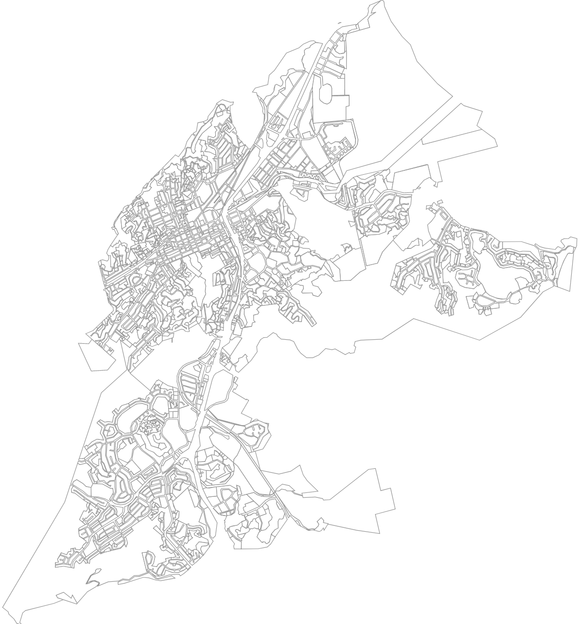
dwg.add(g)Once we generate all the geometries as SVG elements and add them to the instantiate drawing class, then we can save the result:
dwg.save()This will result in a simple, nice, clean vector output:
Adding data attributes
In order to set the attributes, we can initialize the SVG Group element with additional attributes. We can do this by creating a number of additional key/values that are included as “extras” parameters for the SVG Group object.
# Debug set to false to allow alternative attribs keys per inline comment in GH repo:
# mozman/svgwrite/blob/5ce5ed51c094223043644bed7fd89e8d7ccdc91f/svgwrite/base.py#L39-L46
extras = {'debug': False}
for key in row.keys():
    if not key =='geometry':
        extras[f'data-{key}'] = row[key]
g = svgwrite.container.Group(**extras)
You will notice that I also have the debug flag set to false. This was a giant PIA to figure out, but it turns out that this is defaulted to true and the flag is referred to within the element to determine what allowed element attributes are. It’s limited to a hardcoded set unless you turn debug on, in which case this set list is not used or referenced and any element key can be added to an element - so use with caution.
Adding data driven SVG styles
Stylesheet references can easily be added to an SVG. These are reference CSS files and can include information to style an SVG based on data attributes, for example.
Adding them is very straightforward:
dwg.add_stylesheet(stylesheet_loc, 'foo')Once we generate a color generating mechanism for each value in a given dataset (for now we will just look at the zoning column), we can create a template to fill in the categorical styles so that each zoning category has a color associated with it:
# Create a data-driven color scheme based on
custom_style_rules = []
template = r'g[data-zoning="{key:s}"] polygon /\{\{/ fill: {color:s}; /\}\}/'
for key, color in make_color_lookup(gdf, 'zoning').items():
    style_rule = template.format(key=key, color=color)
    custom_style_rules.append(style_rule)
From these results, we can save this new line-delimited string as a CSS file:
stylesheet_loc = f'{fname}.css'
with open(stylesheet_loc, 'w') as f:
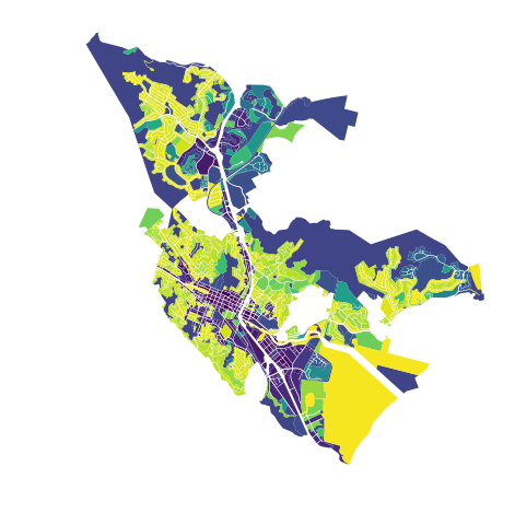
f.write('\n'.join(custom_style_rules))Let’s mimic the viridis matplotlib colormap. When plotting in Geopandas, it is super easy to do this, you just plot the graph and flag which column you want (e.g. “zoning”) and which color ramp you want (e.g. cmap='viridis').
To replicate that, I made a simple method that creates a dictionary of hex values associated with each categorical:
from typing import Dict
import matplotlib
import math

def rgba_to_hex(r):
    i = [math.floor(v * 256) for v in r]
    return '#%02x%02x%02x' % (i[0], i[1], i[2])

def make_color_lookup(gdf: gpd.GeoDataFrame, col: str) -> Dict:
    u = gdf[col].unique()
    l = len(u)
    cmap = matplotlib.cm.get_cmap('viridis')
    normalize = matplotlib.colors.Normalize(vmin=0, vmax=l-1)
    colors = [cmap(normalize(value)) for value in range(l)]

    # Make sure we use the whole color range
    # no colors wasted here, no sir
    assert len(colors) == l

    # Make a lookup dict for the unique vals
    return {z: rgba_to_hex(c) for z, c in zip(u, colors)}
Combining styling, SVG geometries, and data export
We can wrap all the above operations together in a helper method:
import svgwrite

def create_svg_of_gdf(gdf, fname):
    viewbox = ' '.join(map(str, gdf.total_bounds))
    dwg = svgwrite.Drawing(f'{fname}.svg', height='100%', width='100%', viewBox=(viewbox))

    # Default style is plain black outline with white fill
    white = '#FFFFFF'
    grey = '#969696'
    dwg.fill(color=white)
    dwg.stroke(color=grey, width=1)

    # Create a data-driven color scheme based on
    custom_style_rules = []
    template = r'g[data-zoning="{key:s}"] polygon /\{\{/ fill: {color:s}; /\}\}/'
    for key, color in make_color_lookup(gdf, 'zoning').items():
        style_rule = template.format(key=key, color=color)
        custom_style_rules.append(style_rule)

    stylesheet_loc = f'{fname}.css'
    with open(stylesheet_loc, 'w') as f:
        f.write('\n'.join(custom_style_rules))

    dwg.add_stylesheet(stylesheet_loc, 'foo')

    for i, row in gdf.iterrows():
        mp = [[(x, y) for x, y in zip(*g.exterior.coords.xy)] for g in row.geometry]

        # Debug set to false to allow alternative attribs keys per inline comment in GH repo:
        # mozman/svgwrite/blob/5ce5ed51c094223043644bed7fd89e8d7ccdc91f/svgwrite/base.py#L39-L46
        extras = {'debug': False}
        for key in row.keys():
            if not key =='geometry':
                extras[f'data-{key}'] = row[key]
        g = svgwrite.container.Group(**extras)
        for p in mp:
            dp = dwg.polygon(points=p[:-1])
            g.add(dp)
        dwg.add(g)

    # Save the result
    dwg.save()
Calling this method is simple (and saving it, too). Of course this is very rough and could be polished, but it will create 2 files in the local directory: a CSS file and an SVG file that references it.
create_svg_of_gdf(gdf, 'testalt')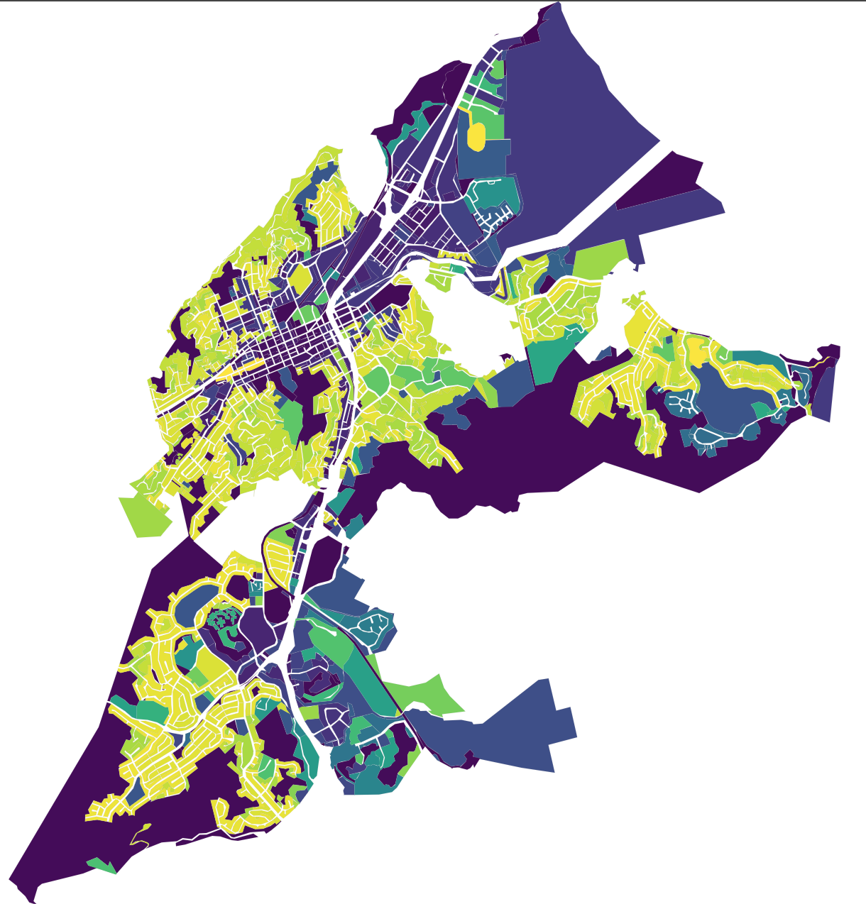
Based on these style rules, the final output SVG will render in a similar fashion to the raster output of the matplotlib plot on from Geopandas built in plot method. Except, this time, it’s in a vector format, which allows for nice things like crisp, high res renders and vector software manipulation (e.g. in something like Adobe Illustrator).
The SVG is viewable on Github as a Gist:
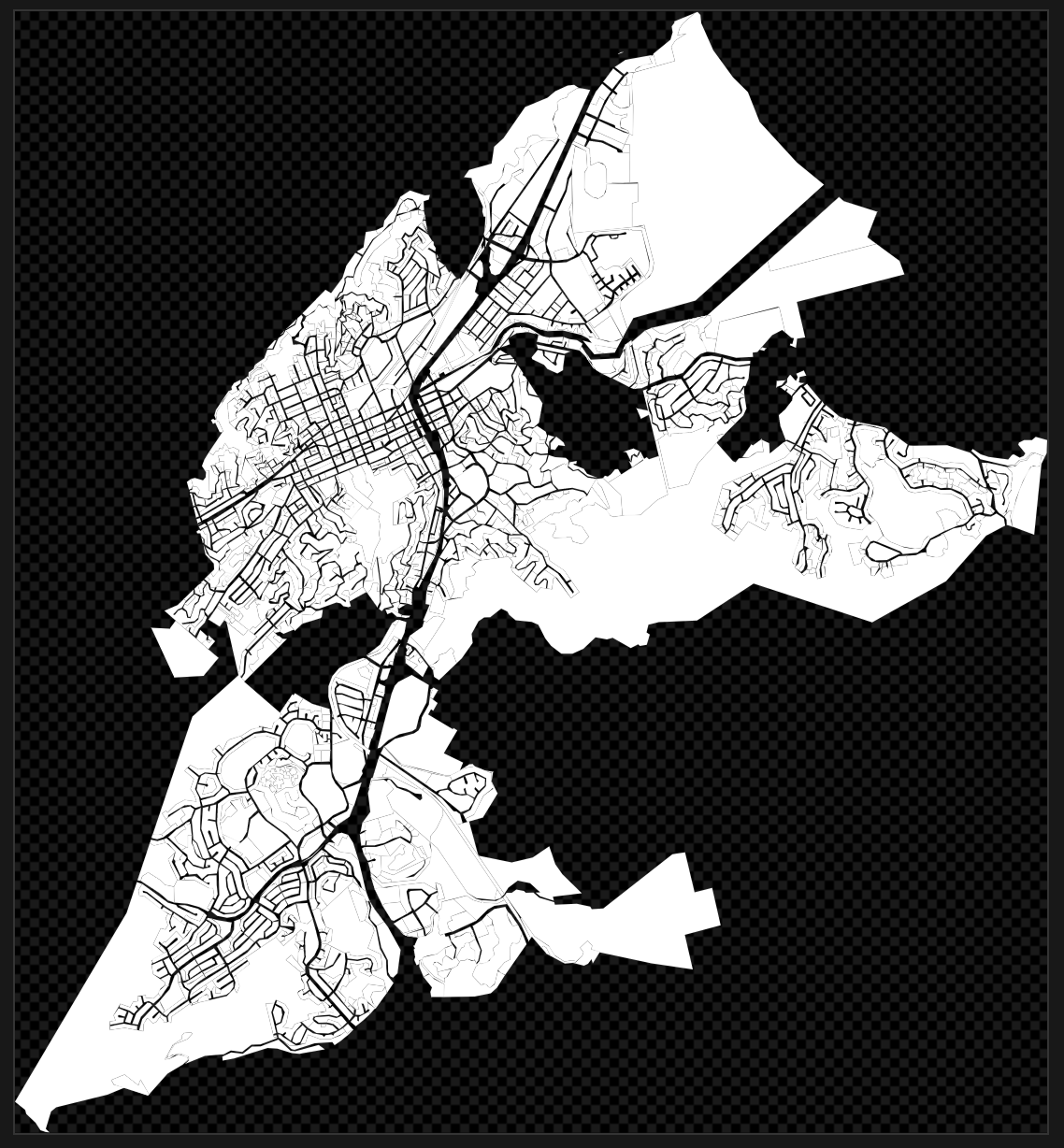
We can also view the resulting components of the SVG at this Gist.
A preview (which won’t load the style right, unfortuantely) is shown below:
