Note: This is the second part in a two-part series. The first section is located here: Programmatic Geometry Manipulation to Auto-generate Route Splines.
This is part of a 4 part series, realted to deep diving into Flocktracker Bogota data. All 4 parts in the series are:
- Cleaning and Analysis of Bogota Flocktracker Data
- Programmatic Geometry Manipulation to Auto-generate Route Splines
- Tethering Schedules to Routes via Trace Data
- Synthesizing Multiple Route Trace Point Clouds
Introduction to Part 2
In this post, we will be working with the same data from the previous post on converting trip trace data to route splines and paired GTFS schedule data. The intent of this post is to sketch out the logic behind how I’ve used the outputs from the route spline generation to auto-generate speed zones along discrete routes and use those to infer time cost which can then be used to generate GTFS for a given route.
When referring to the “current algorithms,” I will be referring to the state of the ft_bogota Github repo I created to support these analyses. The state of the current build of the sketch utility repo when this was written is at commit 10d3a9f5e88e8be36911dd8622ed1a8391d7a3fd. Reviewing the repo after this commit may reveal significant differences. It is important to understand this post more as a proposal with a functional sketch system built out than a finalized implementation of such a utility package.
A notebook that provides something for readers to follow along with exists here as a Gist. I would just like to warn that it’s very much a working document so please excuse the dust. For this post, we will be starting from In [585]. The top of the cell should look like this:
final_costs_gdf = None

for tkey in trip_pairings.keys():
    print('Working on {}'.format(tkey))
    t_list = trip_pairings[tkey]
    t_list.append(tkey)
Introducing the order of operations
The following will be a series of Python operations that are to be run on the output of the trip_pairings dictionary. Essentially, these operations can be wrapped in a method do_something() and executed once for each key in trip_pairings.keys(), with key as an argument variable.
The trip pairings variable was name unique_trip_id_pairs in the previous post and represents all related trip IDs for a given route that has been determined via the route spline generation method (again, from the last post; so please read it first before this post).
Description of initial operations for each key
First we pull pull out the list of valid trip IDs (t_list = trip_pairings[tkey].append(tkey)), where tkey is the key from the trip pairings object whose keys are being iterated over.
We subset the original cleaned Bogota dataset and extract just the related trip ID rows.
# Get subset of dataframe with just the trips from this grouping
trips_set = bdfc[bdfc.trip_id.isin(t_list)]
Now, we are going to create a reference GeoDataFrame. This will hold all trip shapes for this route. Each will have a number of metadata attributes included in their row as well. These will be used to create averages of speed over segments.
Description of internal trip-unique for loop
Just like we did in the last blog post, there’s a fairly long winded segment of this process that lies in a for loop. What I am going to do is show the whole process and tag each step as a “Part.” Each part will then have a subsegment below that outlines what was done there.
# Iterate through the trips and get the speeds for each trip
for target_trip in t_list:

    # Part 1
    single_trip_sub = trips_set[trips_set['trip_id'] == target_trip]
    # Get all lat and lon values from parent dataframe
    single_trip_lon = single_trip_sub['lon'].values
    single_trip_lat = single_trip_sub['lat'].values
    single_tr_xys = [Point(x, y) for x, y in zip(single_trip_lon, single_trip_lat)]
    gdf = gpd.GeoDataFrame(single_trip_sub, geometry=single_tr_xys)

    # Part 2
    dists = [0]
    for a, b in zip(single_tr_xys[:-1], single_tr_xys[1:]):
        d = ft.great_circle_vec(a.y, a.x, b.y, b.x)
        # d is meters and we want km/s
        dists.append(d/1000)
    gdf['segment_distance'] = dists

    # Part 3
    time_delta = (gdf['date'] - gdf['date'].shift()).fillna(0)
    hrs = time_delta.dt.seconds / (60 * 60)

    kmph = np.array(dists)/hrs
    gdf['kmph'] = kmph.fillna(0)

    # Part 4
    # If less than 1 meters moved, speed is 0
    gdf.loc[gdf['segment_distance'] < 0.0001, 'kmph'] = 0.0
    gdf.loc[gdf['kmph'] > 85.0, 'kmph'] = 85.0

    # Part 5
    if final_overall_gdf is None:
        final_overall_gdf = gdf.copy()
    else:
        final_overall_gdf.append(gdf)
Part 1
Here, we convert the subsetted data frame of only relevant trip IDs and iterate through each unique trip ID in that list. For each, we first convert that into a single GeoDataFrame of just that trip. We can then get the distance between each point.
Part 2
In this step, we take all those Shapely Points and calculate the distance between each for the trip. Note that this data frame is already sorted by date, which is why we do not need to sort it again. The zip method will be successful because each subsequent point comes “after” the preceding in terms of the time they were logged.
Part 3
Similarly, we can use the Pandas .shift() method to get the time difference between each point. In the case of the Bogota data, they should all be 5 seconds apart, but this allows for the possibility that there may have been some technical error that caused one point to be omitted.
Once we have the time difference data, we can also calculate the speed by using the distance data from Part 2. This, the distance data itself, and the time are all added to the parent GeoDataFrame.
Part 4
With the resulting GeoDataFrame, we want to make sure we do not have ridiculous results. Thresholds have been set to prevent any points from exhibiting excessive speeds. That said, this should not occur because I have cleaned the Bogota data and removed all outliers.
Part 5
With this cleaned and prepared GeoDataFrame, we can update the final_overall_gdf reference by appending these new rows of processed trace data.
Identifying speed zones
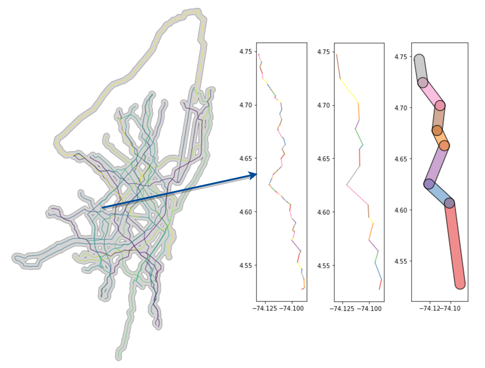
At this point we want to get the route LineString shape for the target route. We want that and we simplify it. In the case of the degrees-projected Bogota dataset, we simplified by 0.0025:
# Now pair these values back to points on the main routes LineString
ls = routes_gdf[routes_gdf.id == tkey].path.values[0]
coords = [c for c in ls.simplify(0.0025).coords]
With these results, we can a bunch of discrete segments (as shown in the image above).
broken_up_ls = []
for a, b in zip(coords[:-1], coords[1:]):
    broken_up_ls.append(LineString([a, b]))
With each of these buffered segments (as shown, buffered, in the rightmost plot above), we can then get descriptive stats for all speeds in that zone:
speed_for_seg = []
for l in broken_up_ls:
    l_buff = l.buffer(0.005)

    overall_sub = final_overall_gdf[final_overall_gdf.intersects(l_buff)]
    kmph = overall_sub.kmph

    medi = kmph.median()
    mean = kmph.mean()

    speed = medi
    if medi > mean:
        speed += medi - mean
    else:
        speed += mean - medi

    if np.isnan(speed):
        speed = 0
    speed_for_seg.append(speed)
In the above code snippet, I iterate through all rows from the prepared trip traces and pull out those that are in the speed zone. I take the mean and median and use the average between the two as the speed for that segment. This could be changed to however you as a user feel would generate a most appropriate descriptive speed for this zone. Depending on the amount of data that you have on hand, you could also do a peak hour and off peak hour speed for that leg of the route journey. In my case, all times are assumed peak.
Generating final costs
Remember that final_costs_gdf reference from the very beginning? Let’s begin to populate it.
First, we need to create a number of reference lists.
orig_pts = []
p_xs = []
p_ys = []
trip_ids = []

p_speeds = []
p_dists = []
p_time_costs = []
Each of the above lists will become a column in the resulting GeoDataFrame. The first 4 are all related to the original route points (which we will use as stops), their coordinates, and the trip ID they are paired with.
In the next segment, we iterate through the LineString and update the route shape reference as a GeoDataFrame with the summary speed and time costs between each of those coordinate points (stops for the GTFS).
for c in ls.coords:
    p = Point(c)

    orig_pts.append(p)
    p_xs.append(p.x)
    p_ys.append(p.y)
    trip_ids.append(tkey)

    p_speed = 0
    for i, l in enumerate(broken_up_ls):
        if p.intersects(l):
            p_speed = speed_for_seg[i]
            break
    p_speeds.append(p_speed)

    # Given that speed, figure out the time difference
    # from the last point to the current
    if len(orig_pts) == 1:
        p_dists.append(0)
        p_time_costs.append(0)
    elif p_speed == 0.0:
        p_dists.append(0)
        p_time_costs.append(0.00139) # 5 seconds
    else:
        # Calculate the distance in km
        a = orig_pts[-2]
        d = ft.great_circle_vec(a.y, a.x, p.y, p.x)
        km = d/1000
        p_dists.append(km)

        # And the time cost between two points
        # Time in portion of an hour
        p_time_cost = (1/p_speed) * km
        p_time_costs.append(p_time_cost)

    pt_sums = np.array(p_time_costs)
    pt_sums[np.isnan(pt_sums)] = 0

    pd_sums = np.array(p_dists)
    pd_sums[np.isnan(pd_sums)] = 0

    new_gdf_to_append = pd.DataFrame({
        'trip_id': trip_ids,
        'x': p_xs,
        'y': p_ys,
        'speed': p_speeds,
        'seg_distance': pd_sums,
        'time_cost': pt_sums,
        'order': np.arange(len(trip_ids)),
        'geometry': orig_pts
    })
In an attempt at quality control, we only add to final_costs_gdf if the total length is of a significant distance and is not just someone turning the app on by accident and walking around at the start of finish of their route trip by accident.
# Don't even record "mini-routes" that slip through
if pd_sums.sum() > 0.05:
    if final_costs_gdf is None:
        final_costs_gdf = new_gdf_to_append
    else:
        final_costs_gdf = final_costs_gdf.append(new_gdf_to_append, ignore_index=True)
An improvement that could be made here is to have intermediary stops along the line segments if they exceed a certain distance. I could actually introduce this upstream by taking the simplified geometry and breaking up component lines that are over a certain length threshold.
Generating the GTFS
Now that we have the time cost calculated for each of the routes, converting this into GTFS is pretty straightforward and more a matter of just complying with the GTFS format. In the following sections, I’ll show how to generate each of the required files and include any relevant notes.
Stops table
Again, we use the trip ID as the unique ID for a give route and just strip the “T” from the name. “X” and “Y” coordinate values were already broken out from the LineString in the above section’s for loop.
stops_df = final_costs_gdf.copy()
stops_df['stop_id'] = stops_df['trip_id'].str.replace('T', '') + '_' + stops_df['order'].astype(str)
stops_df['stop_name'] = stops_df['stop_id'].copy()
stops_df['stop_lat'] = stops_df['x'].copy()
stops_df['stop_lon'] = stops_df['y'].copy()

stops_df = stops_df[['stop_id', 'stop_name', 'stop_lat', 'stop_lon']]
stops_df.to_csv('../bogota_stops.csv', index=False)
Routes table
Generating routes tables is also straightforward and more a matter of making sure that naming conventions are consistent with the other tables. I’ve put all these informal routes under the same operator, hardcoded as “FT_BOGOTA”. There is no informal bus route type, so they all were designated the standard bus type 3 for GTFS.
routes_df = final_costs_gdf.copy()
routes_df['route_id'] = routes_df['trip_id'].str.replace('T', '')
routes_df['agency_id'] = 'FT_BOGOTA'
routes_df['route_short_name'] = routes_df['route_id'].copy()
routes_df['route_long_name'] = routes_df['route_id'].copy()
routes_df['route_type'] = 3

routes_df = routes_df[['route_id', 'agency_id', 'route_short_name', 'route_long_name', 'route_type']]
routes_df = routes_df.drop_duplicates()
routes_df.to_csv('../bogota_routes.csv', index=False)
Shapes table
This table is easier than it might seem. All that needed to be done is to add each LineString point as a row in the data frame and link it to the route (and also add sequence number).
shapes_dict = {
    'shape_id': [],
    'shape_pt_lat': [],
    'shape_pt_lon': [],
    'shape_pt_sequence': [],
}

for i, row in routes_gdf[['id', 'path', 'service_area']].iterrows():
    sh_id = row.id.replace('T', '') + '_shp'
    seq = 1
    for p in row.path.coords:
        pt = Point(p)

        shapes_dict['shape_id'].append(sh_id)
        shapes_dict['shape_pt_lat'].append(pt.y)
        shapes_dict['shape_pt_lon'].append(pt.x)
        shapes_dict['shape_pt_sequence'].append(seq)

        seq += 1

pd.DataFrame(shapes_dict).to_csv('../bogota_shapes.csv', index=False)
Calendar table
Because we do not have enough data about operation, the calendar data just assumes a “GENERIC” default of having service every day for all routes.
calendar_dict = {
    'service_id': ['GENERIC'],
    'monday': [1],
    'tuesday': [1],
    'wednesday': [1],
    'thursday': [1],
    'friday': [1],
    'saturday': [1],
    'sunday': [1],
    'start_date': [20170101],
    'end_date': [20190101],
}

pd.DataFrame(shapes_dict).to_csv('../bogota_calendar.csv', index=False)
Trips and Stop Times table
These are the only complex tables to create. They need to be generated in tandem because each trip needs to be paired with a unique schedule of arrivals and departures from all stops. As a result, for each new trip entry in the trips table, we need to create all relevant stops arrivals for the stops table under that trip ID.
The below is the entire workflow. The loop should be fairly straightforward. You will notice that I’ve only produced one hour (8:00 AM) of stop time data. This could be adjusted according to what window you wanted to generate data for. Naturally, these aspects could be parameterized and all wrapped in a more clean generator function. Before that is built though, more consideration needs to be directed at thinking about how to handle different schedules for different routes based on more robust observation data (e.g. data covering a single trip or route over multiple days and on weekdays and weekends).
trips_dict = {
    'route_id': [],
    'service_id': [], # always GENERIC
    'trip_id': [],
    'direction_id': [],
    'shape_id': [],
}

stop_times_dict = {
    'trip_id': [],
    'arrival_time': [],
    'departure_time': [],
    'stop_id': [],
    'stop_sequence': [],
}

for tid in list(set(routes_gdf.id.values)):
    print('Working on {}'.format(tid))
    route_id = tid.replace('T', '')
    service_id = 'GENERIC'
    trip_id = None
    shape_id = route_id + '_shp'

    arrival_time = None
    departure_time = None
    stop_id = None
    stop_sequence = None

    trip_num = 1

    # this will do one trip every 5 minutes
    for i in range(12):
        sub = final_costs_gdf[final_costs_gdf.trip_id == tid]

        for direction in [0, 1]:
            trip_id = route_id + '_' + str(trip_num)
            trip_num += 1

            trips_dict['route_id'].append(route_id)
            trips_dict['service_id'].append(service_id)
            trips_dict['trip_id'].append(trip_id)
            trips_dict['direction_id'].append(direction)
            trips_dict['shape_id'].append(shape_id)

            # Note: Only will generate for 1 representative hour (8:00 AM)
            start_time = '08:00:00'
            start_hr = 8
            start_min = 0 + (i * 5)
            start_sec = 0

            if direction == 0:
                sub = sub.sort_values(by='order', axis=0, ascending=False).reset_index(drop=True)
            else:
                sub = sub.sort_values(by='order', axis=0, ascending=True).reset_index(drop=True)

            for i, row in sub.iterrows():
                added_time = row.time_cost * 60

                if (added_time > 0) or (i == 0):
                    new_min = round(added_time, 0)
                    new_sec = round(((added_time % 1) * 60), 0)

                    # update min and sec values from parent scope
                    start_min = new_min
                    new_sec = new_sec

                    hr = start_hr
                    if hr < 10:
                        hr = '0' + str(hr)
                    hr = str(hr)

                    minute = start_min
                    if minute < 10:
                        minute = '0' + str(minute)
                    minute = str(minute)

                    # Follow string formatting for time
                    sec = start_sec
                    if sec < 10:
                        sec = '0' + str(sec)
                    sec = str(sec)

                    arrival_time = ':'.join([hr, minute, sec])
                    departure_time = arrival_time
                    stop_id = route_id + '_' + str(i)
                    stop_sequence = i

                    stop_times_dict['trip_id'].append(trip_id)
                    stop_times_dict['arrival_time'].append(arrival_time)
                    stop_times_dict['departure_time'].append(departure_time)
                    stop_times_dict['stop_id'].append(stop_id)
                    stop_times_dict['stop_sequence'].append(stop_sequence)
Closing thoughts
The GTFS generation is still rickety but, as I hope is clear from this post, is pretty straightforward once we have the route data. I’d say that it is the route shape data that is most critical. Once we know where the routes are, getting and refining a schedule for these shapes is more a matter of data than a technical challenge generating discrete references from an assemblage of partial data.
If you made it this far, thanks for reading!
This is part of a 4 part series, realted to deep diving into Flocktracker Bogota data. All 4 parts in the series are: