Synthesizing Multiple Route Trace Point Clouds

Introduction

In the following post I describe a quick and dirty method for taking the traces from multiple trips and imputing a likely spline from the point cloud. The advantage of this method is that no order is needed for the original trace points. This means that we can combine multiple trips together that ran along the same route, as well as include trips that did not run the entire segment of the other trips.

This is part of a 4 part series, realted to deep diving into Flocktracker Bogota data. All 4 parts in the series are:

• Cleaning and Analysis of Bogota Flocktracker Data
• Programmatic Geometry Manipulation to Auto-generate Route Splines
• Tethering Schedules to Routes via Trace Data
• Synthesizing Multiple Route Trace Point Clouds

Example use case

What would be a use case for this? Say you are mapping transit routes and you have volunteers performing the tracing using cell phones. They may not all ride the trip at the same time, nor may they all ride the same trip from start to finish. Furthermore, some may ride it one way and some another. Typically, it would be difficult to combine these trips and try to impute a single route from them.

With the method I outline, one can combine all available traces related to a given route and then merge the point clouds together. From the combined point cloud a single LineString object is returned. With this object, we can then easily convert the shape to GeoJSON and either submit it as-is or run it through a map matching service like Mapzen’s Flex API. This will snap the route to existing OpenStreetMap (OSM) paths. Also, we can take the resulting LineString information and pin nodes to it to generate standardized GTFS data. This is important for creating stating schedule feeds as a core requirement of GTFS is a reference route path.

Running through the process

Let’s start with an example spread of data. In this example, notice that there is a clear path for the data but there is scattershot accuracy. The above image features a zoomed-in segment of one leg of the total combined traces. A clear direction and trajectory is visible from the unsorted point cloud of data, by looking at it visually. A bounds has been drawn around the data and we can see that, although it is a multipolygon, it roughly follows the path of an (as of yet not determined) spine.

First, merge all points from all traces into a single array composed of Shapely Points objects. Buffer these according to the resolution of the GPS signal as observed (e.g. 50 meter accuracy so buffer all points by 50 meters).

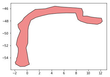
Once buffered, we should be able to unary union the result to a single blog like shape, as in the above example image.

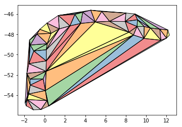
We can use Shapely’s built in triangulate method to create triangle planes between all existing vertices from the polygon’s coordinates. If you want to more about triangulation, check out my previous post on constrained vertices and Delaunay triangulation methods. The script would be as follows:

from shapely.geometry import MultiPolygon
from shapely.ops import triangulate

triangles = MultiPolygon(triangulate(shape, tolerance=0.0))

Now let’s drop all triangles that fall outside of the bounds of the original, parent shape.

The result, as seen above, is fairly straightforward and is created via the following:

tri_cleaned = []

# only preserve the triangles that are within the bounds
# of the parent shape
for poly in triangles:
    if poly.centroid.intersects(shape):
        tri_cleaned.append(poly)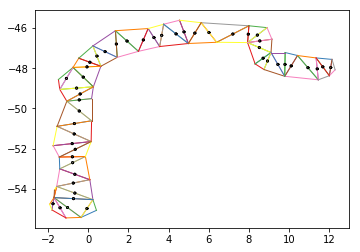

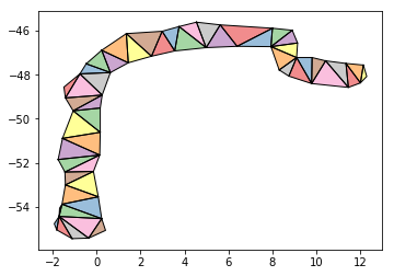
Now comes the fun part. We need to break this shape down into its component vertices and extract the midpoints of only those that are not along the edges/exterior of the shape. The result, plotted, should look like the above. Below, a script hashes out a quick way to accomplish this:

from shapely.geometry import Point, LineString

lines_and_points = []
just_points = []

# used as reference
shape_buff = shape.exterior.buffer(.1)

# extract the midpoints of all triangles in the triangulated point
# cloud shape that do not reside on the geometry exterior
for tri in tri_cleaned:
    ext = tri.exterior.coords
    for start, fini in zip(ext[:-1], ext[1:]):
        lines_and_points.append(LineString([start, fini]))

    for start, fini in zip(ext[:-1], ext[1:]):
        pt_0 = start[0] + ((fini[0] - start[0])/2)
        pt_1 = start[1] + ((fini[1] - start[1])/2)

        new_pt = Point([pt_0, pt_1])
        new_pt_buff = new_pt.buffer(.05)

        
        if not new_pt.intersects(shape_buff):
            lines_and_points.append(new_pt_buff)
            just_points.append(new_pt)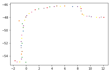

Great, now we have all the points that we need to work with. As you can see in the above image, these points roughly make the “spine” of the geometry. They are in no particular order, though.

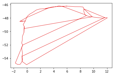
We can see how out of order they are by plotting them as a LineString, as in the above. Naturally, the triangulation method creates no “start to finish” order, so we must infer one. Because we have a structured point cloud now, though, where each point roughly correlates with one point along the spine of the geometry, we only need two pieces of information to be able to infer the order of the line.

First, we need the start point and then we need the end point. We can get these from any trip that has both of them. In our case, so long as one rider has done the whole trip we can do this by pulling that rider’s first and last points. We can select the longest route of all “complete” rides in order to access these reference start and end points.

Once we have them, getting the start and end points is merely a matter of getting the nearest point in the midpoint vertices point cloud to each of them.

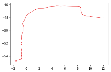
Once we have them, we can iterate through the remaining midpoint points, finding each subsequent closest point from the start point, until we reach the end point. Doing so will create a sorted line for us, as we can see in the above image.

We can see the process for achieving that in the below script:

remaining = copy.copy(just_points)
sorted_pts = [start_pt]

reached_end_pt = False

while not reached_end_pt:
    current = sorted_pts[-1]
    nearest = None
    dist = 10000
    for pr in remaining:
        d = pr.distance(current)
        if d < dist:
            nearest = pr
            dist = d
    
    sorted_pts.append(nearest)
    remaining.remove(nearest)
    
    # check if this is the same as the end pt
    if list(nearest.coords) == list(end_pt.coords):
        reached_end_pt = True

Methodology limitations

This is by no means the most refined method of inferring a point cloud spline but it’s fast and dirty. With additional tools like Mapzen’s map matching tools, this method will get you “close enough” so that the final refinement against OSM path network data is possible. It will also leverage the advantages that multiple crowd-sourced pass throughs of a given route affords. That is, we can normalize against noise and discrepancies on multiple rides. Ends of rides may still be a little awkward so some further refinement may be necessary to handle the “hooks” that can occur (as seen in the above example). That said, map-matching typically handles such issues sufficiently to produce useful final shapefiles, which can be used as reference route shapes for any downstream analysis or scheduling, such as in creating a GTFS schedule.

from geojson import LineString as gj_LineString
gj_LineString(list(LineString(sorted_pts).coords))

# returns
# {"coordinates": [[-1.021728515625, -54.92412823402425],
# [-1.021728515625,
# …
# -47.9291803556701],
# [12.06298828125, -47.96627422845168]], 
# "type": "LineString"}

For reference, here’s a notebook of the steps taken in the above blog post: Gist.

Update dealing with limitations during a real world example

Unfortunately, this method is not as rock solid as I initially thought. Below are some screen captures from me running through this method with a real dataset from the Flocktracker Bogota data. For those who have access to the data, I was using Trip ID T49774371.

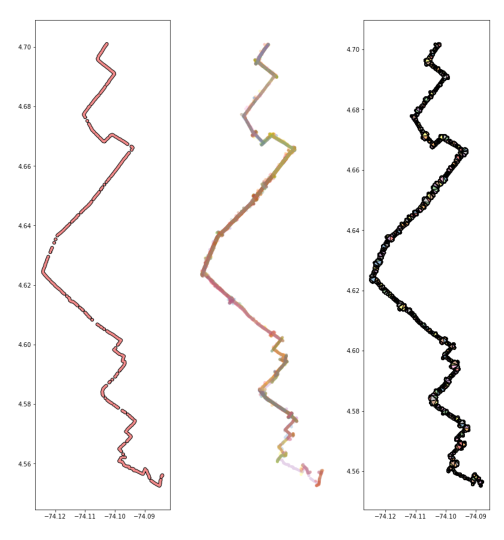
Trip T49774371 is shown in the first image above. The second, middle one, is the result of all trips merged that overlap with that trip. As you can see, this is an effective way of capturing all the trips that run along the same route.

Once we pull in all those similar trips, we can merge them into a single shape and triangulate it. As you can see in the right most image above, that shape is very complex.

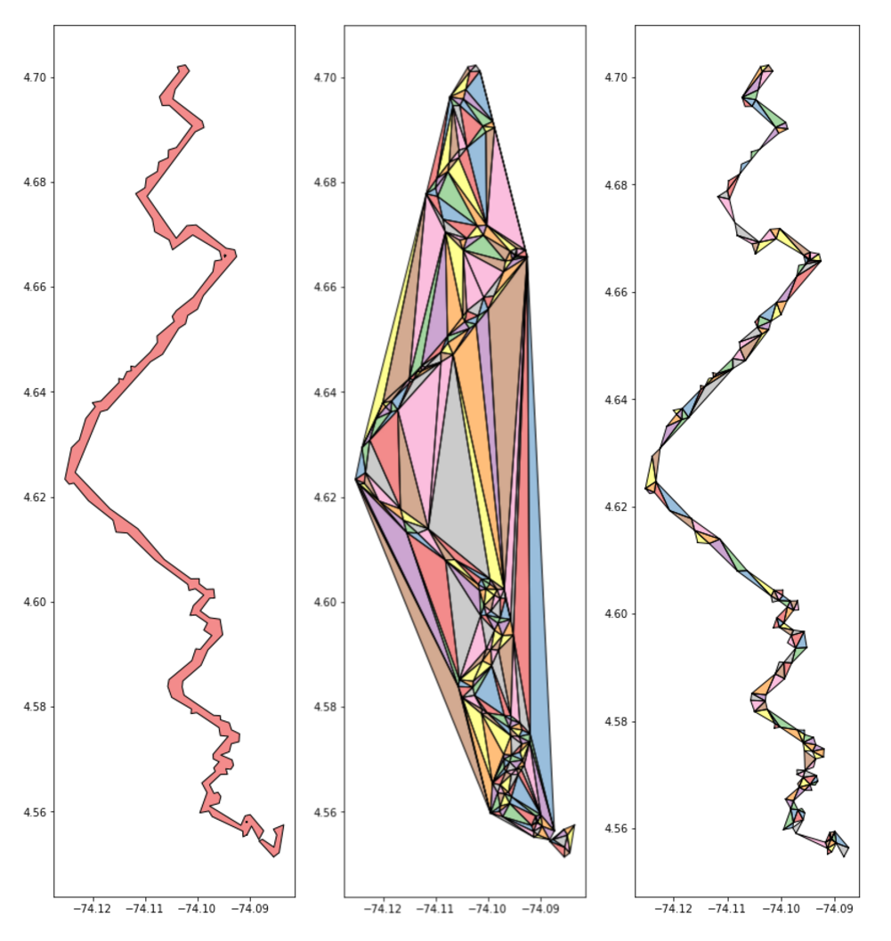
We can take a step back and simplify that original unary union of buffered points (50 meter buffer as GPS trace accuracy roughly matches that). In the following steps we perform a simple triangulation operation and plot the results of this simplified geometry. The operation is much fast as the number of triangles has been reduced by about an order of magnitude.

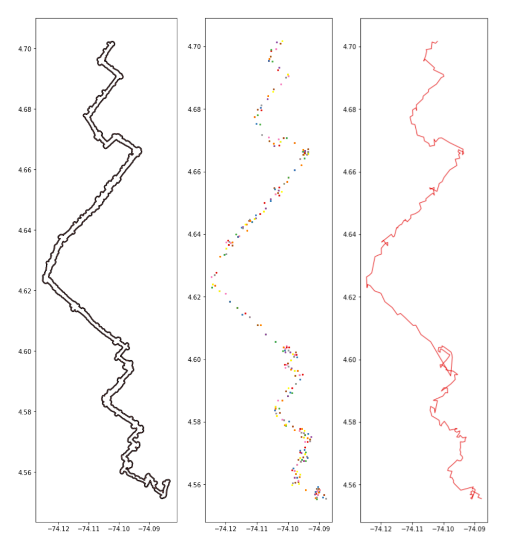
This leads us to the third series of operations. Here, we parse out all points from the midpoints of those triangle vertices that touch the edges of the buffered route shape. From that resulting point cloud we try and tease out a path that should be the spline.

Here’s where this methodology starts falling apart. The mess about 30% up from the southernmost point of the route is causing trouble. In these areas, we can see that the methodology failed to handle the tight turns in the route.

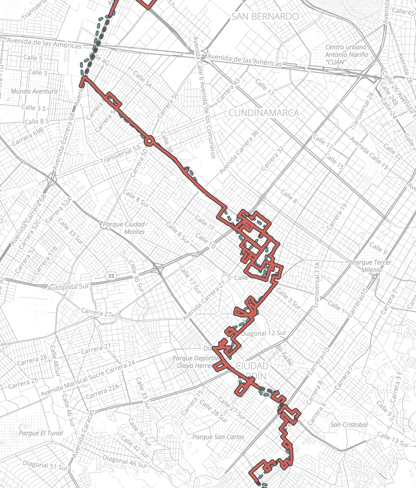
We can see how complex this part of the network is when we look at the map match results as well. Mapzen Flex does its best to pair these squiggles with the road network, but the result is a hair ball of paths.

As a result of this exploration, it is clear I will need to work on a better method of cleaning these splines so that we can manage these complex routes. One strategy may be to just dump the portions of the path that loop on themselves by pinpointing the self intersection and dropping all points between it. This could have some unforeseen consequences, though. I will report back here with any learnings when they occur/are discovered.

Second Update: Using shortest path to impute a rough spine

After working on this for some time, I’ve come to the conclusion that it might be best to simply accept at first that the GTFS does not match the street network. This is a defensible position for the following reasons:

• Many GTFS feeds do not provide high resolution shapefiles of the routes
• In fact, shapefiles are not a required component of the core GTFS feed
• What is important is static stop points
• Because we have clusters that can help us identify where stops occur, we now need only to focus on that and the path between those key points can be a rough approximation

With this in mind, I propose a new method of determining the rough spine of a given route, and a method that will be guaranteed to be off - but not by much. More importantly, it will be within a marging of error that will allow for the moving forward of analysis on service shed coverage and the generation of rudimentary GTFS schedule data.

The below three images should help visualize the methodology being proposed. A discussion of it will follow, below them.

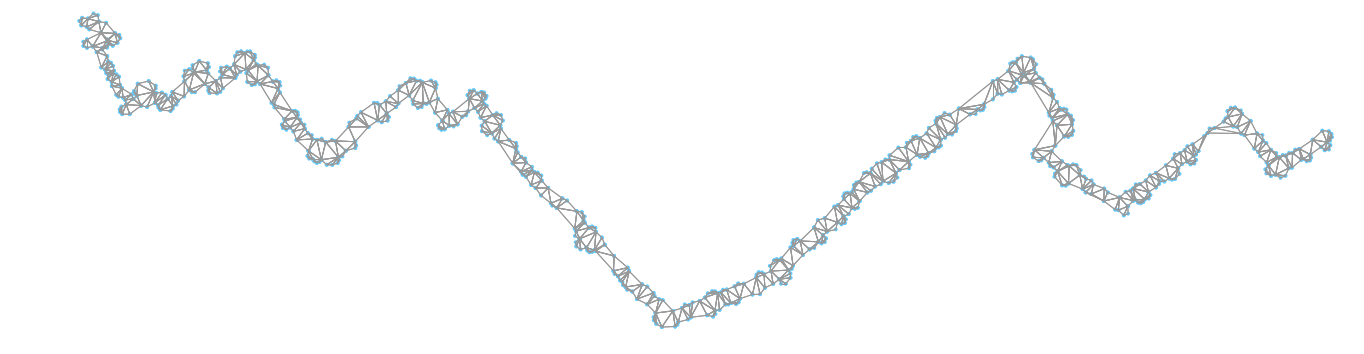
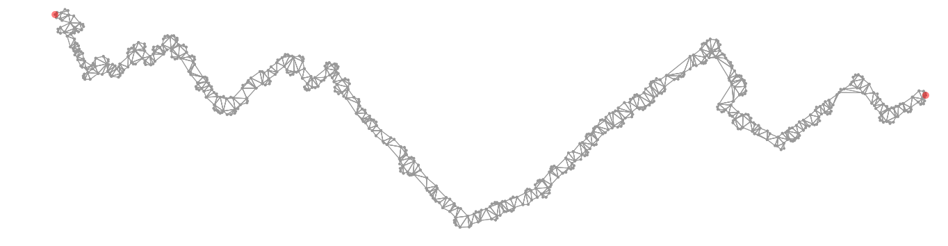
The above steps are similar to the intial steps we have taken prior. The difference is that, once we have triangulated the buffered consolidated geometries (top image) and inferred the start and end points (second image), we now convert that triangulated shape itself in to a network graph.

This allows us to traverse the new shape and find the shortest path within its vertices from the start point to the end point.

Using NetworkX, I convert the vertices of each triangle to edges in an network. The coordinates themselves are then manifested as network nodes. A sloppy execution of this method is as follows:

import networkx as nx
G = nx.MultiDiGraph()

node_count = 0

id_of_end_pt = None
id_of_start_pt = None

for tri in tri_cleaned:
    coords = list(tri.exterior.coords)

    ids = list(map(lambda x: node_count + x, [1, 2, 3]))
    
    for one_id, coord in zip(ids, coords[0:3]):
        
        thresh = 0.0001
        if end_pt.distance(Point(*coord)) < thresh:
            id_of_end_pt = one_id
        if start_pt.distance(Point(*coord)) < thresh:
            id_of_start_pt = one_id
            
        G.add_node(one_id, y=coord[0], x=coord[1])

    for a, b, i in zip(coords[:-1], coords[1:], ids):
        d = great_circle_vec(a[1], a[0], b[1], b[0])

        a_id = i
        b_id = i + 1

        if b_id > ids[-1]:
            b_id = ids[0]

        G.add_edge(a_id, b_id, length = d)
        G.add_edge(b_id, a_id, length = d)

    node_count += 4

This method above also captures the nearest nodes to the already identified start and end points.

With that, we now have a series of disconnected networks that represent each triangle. We need to make a no-cost edge also for each set of nodes that are identical from one triangle coordinate to another. Again, a quick and dirty example of this:

nodes_as_pts = []
node_ids = []

for node_id, xy in G.nodes(data=True):
    nodes_as_pts.append(Point(xy['x'], xy['y']))
    node_ids.append(node_id)

node_gdf = gpd.GeoDataFrame(node_ids, geometry=nodes_as_pts, columns=['node_id'])
    
for node_id, xy in G.nodes(data=True):
    node_pt = Point(xy['x'], xy['y'])
    ds = node_gdf.distance(node_pt)
    sub = node_gdf[ds < 0.0001]
    
    for to_id in sub['node_id'].values:
        G.add_edge(node_id, to_id, length = 0.00001)
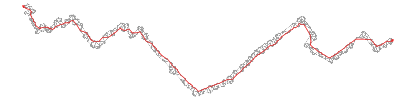
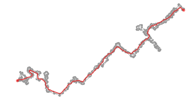
        G.add_edge(to_id, node_id, length = 0.00001)

At this point the final image (bottom) can be generated by identifying the shortest path through this network. The below NetworkX API call will utilize Dijkstra’s algorithm to compute the shortest path within this network, which gives us a reasonable path that avoids the confusion of complex or looping corner cases as we saw in this example. A downside of this is that it fails to capture inlets (such as if a bus were to go into a shopping center and then back out).

route = nx.shortest_path(G, source=21, target=33, weight='length')

For the sake of creating rudimentary GTFS network shapes, though, this method should suffice. Additional coverage area lost can then be recaptured by simply utilizing the point cloud of trace data as a spatial overlay over geometry layers with relevant metata.

Operationalizing the final method

This is a third and final update to this post. The steps to perform this operation are currently being contained into well-scoped methods. I’ll roll all these utilities up into a single utility file. For now, as I am sketching them out, I have called the file flocktracker.py. By importing it, methods can be called quickly and succinctly, like so:

import flocktracker as ft

# first get a single trip (iterate through a list of reference trips
# to then create a GTFS shapes reference for the whole recordings dataset)
target_trip = ft.get_next_target_trip(bdfc, use_vals)
print('Using this target trip: {}'.format(target_trip))

single_trip_mpoly = ft.extract_single_trip(bdfc, target_trip)
grouped_trips = ft.get_similar_routes(single_trip_mpoly, bdfc)

# and so on...

Thus far, this method has been holding up quite well. Here’s another example showing how the operation handled the fact that a route tended to also diverge from the center/main trajectory and go deep into two side streets (below image).

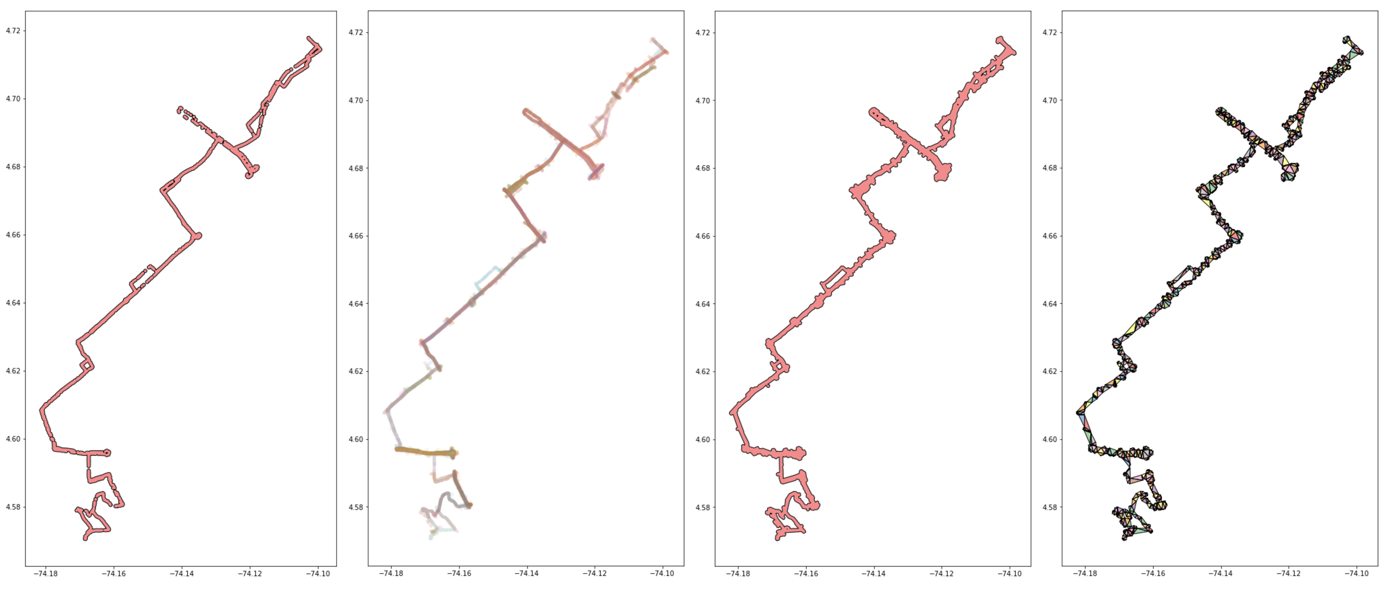
From left to right:

• Starting reference trip
• All overlapping trips
• Simplification step
• Triangulation step

With the current method, we are able to avoid them, but to account for their popularity when determining the speed at which the vehicle should be scheduled to traverse the network. We can effectively “slow down” its performance at this juncture, to acknowledge that it tends to “go off course” at this point and thus those who are farther down the route from this point may have to wait longer than if the vehicle were to consistently go straight on and not diverge.

Aside: It is also possible that this is a situation where there was a segment of another trip that passed through this trip and this small segment was getting caught in this particular route’s traces during the intersection subsetting step. If that is the case, this is another example where the shortest path method comes in handy as a way of handling such situations and ignoring perpendicular intersections to the main route spline.

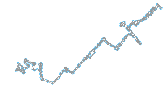
Just as with the prior example, here is the triangulated path, simplified, and converted into a network. The second image is then that same graph but with the shortest path from start to finish superimposed.

Next steps

In addition to finishing up this flocktracker.py utility library, I will need to figure out a way to programmatically determine the start and end nodes for the routes. This is extra tricky as I have noticed that some riders would start in the middle of a route and not at one of its extermities. This makes it hard to be sure that the earliest traces from a trip are at the start or end of the trip. As a result, I will need to devise an alternative strategy for determining route start and end points.

This is part of a 4 part series, realted to deep diving into Flocktracker Bogota data. All 4 parts in the series are:

• Cleaning and Analysis of Bogota Flocktracker Data
• Programmatic Geometry Manipulation to Auto-generate Route Splines
• Tethering Schedules to Routes via Trace Data
• Synthesizing Multiple Route Trace Point Clouds