Note: This is the first part in a two-part series. The second section is located here: Tethering Schedules to Routes via Trace Data.

This is part of a 4 part series, realted to deep diving into Flocktracker Bogota data. All 4 parts in the series are:

• Cleaning and Analysis of Bogota Flocktracker Data
• Programmatic Geometry Manipulation to Auto-generate Route Splines
• Tethering Schedules to Routes via Trace Data
• Synthesizing Multiple Route Trace Point Clouds

Introduction to Part 1

The intent of this post is to outline how previous explorations into converting unsorted points into single route splines has been organized into a workflow that would enable one to generate a GTFS schedule and paired route shape files dataset given minimal trace data. It will also go into where the current algorithms are overly brittle and how such limitations would be remedied in a more robust implementation (or refactor).

When referring to the “current algorithms,” I will be referring to the state of the ft_bogota Github repo I created to support these analyses. The state of the current build of the sketch utility repo when this was written is at commit 10d3a9f5e88e8be36911dd8622ed1a8391d7a3fd. Reviewing the repo after this commit may reveal significant differences. It is important to understand this post more as a proposal with a functional sketch system built out than a finalized implementation of such a utility package.

A notebook that provides something for readers to follow along with exists here as a Gist. I would just like to warn that it’s very much a working document so please excuse the dust.

Context for challenge

Researchers used a tool called Flocktracker (I happened to work on it at MIT a few years ago as a graduate student), to track informal transit routes throughout Bogota, Colombia. Similar studies have been performed from Dhaka, Bangladesh to Mexico City, Mexico. What makes the Bogota study noteworthy is that it was very complete, generating data that covers almost the entire city.

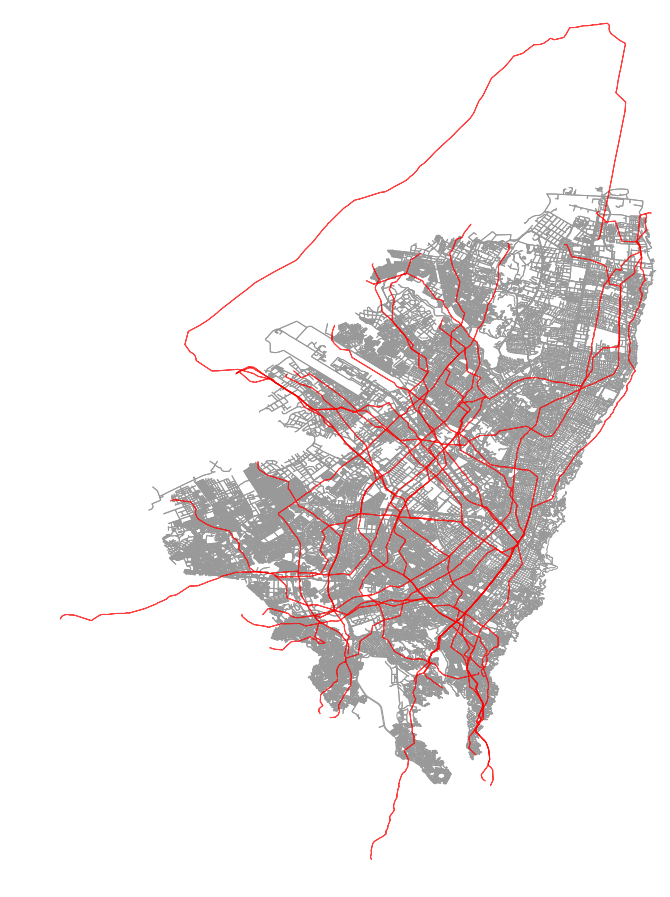
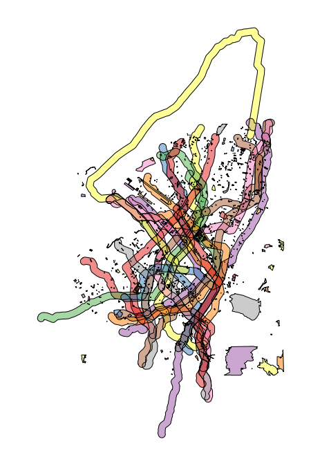
In the above image, we can see the route splines imputed from the original trace point cloud. Using the method outlines in this blog post, I was able to determine that roughly 64.5% of the total area of the city was covered by regular informal transit service. By combining this with population weighted urban planning zone (UPZ) data (Bogota’s rough equivalent of a Census Block Group), and greenspace layer data, I was able to estimate that nearly 60% of the population was serviced by these same routes. The methodology for how this was accomplished will also be outlined in this post.

Overview of the problem

While data from Flocktracker was used, the methods outlined here are in no way exclusive to that tool. Rather, that tool generated data with the following values:

• Unique ID designation a unique trip
• Latitude
• Longitude
• Time stamp for each point crumb

Other data was included, as well, such as rider identification. That said, none of that was necessary. So long as we have traces from trips, no other information is necessary to generate this GTFS.

What’s neat about this is that we open up the possibility for individuals to contribute in a more lightweight way. That is, users could simply supply trace data from their segment of the route and they would not even need to log what route they were on. Their data would be relatively anonymous and, when combined with hundreds of other trips throughout the city, discreet routes could be imputed and a GTFS schedule generated based off these numerous partial observations.

Introduction to utilities library

The methods described in this blog post are being saved in this repo. While the repo may change in time, the overall flow of the operations is being preserved here in code snippets.

At the time of this writing, the utilities library is complete through the generation of unique route shapes. The GTFS generation step has not yet been integrated, but is sketched out in a notebook and will be included in snippets here.

Operations workflow

First, let’s profile the data. In this case, we will work with the Flocktracker Bogota data.

# load in the base csv
bdf = pd.read_csv('../bogota_points.csv')
coords = (-74.421387,4.4,-73.773193,4.957563)
bdfc = ft.clean_base_df(bdf, coords)

# 6408 bad data points out of 510680 total; or 1.25%. 25 out of bounds data points. # Number of unique trip IDs: 388

The ft.clean_base_df method performs a few key functions. First, it pulls out the above mentioned required columns. Critically, it requires the time column (date), location (lon, lat), and unique identified (trip_id). The date column is converted into Pandas’ date time column format.

Null values are dropped and removed, as well all values that lie outside of the supplied bounding box. The bounding box is a rough bounding of the Bogota area. The primary intent for this operation is to drop wildly off coordinates. This occasionally, happens, and often points can end up on Null Island, the default coordinate location that a phone may supply as its location when it is unable to successfully calibrate itself.

Once we have the unique trips pulled out and cleaned (held in bdfc, a shorthand for “Bogota Data Frame Clean”), we need to create two output dictionaries:

# We will use this to hold all our final result shapes
unique_trip_paths = {}
unique_trip_id_pairs = {}

What these represent are the final output values. We will be iterating through an order of operations and the result of this iteration will be cleaned route geometries placed in the above reference dictionaries.

The loop we will be creating will be iterating through all the resulting unique trip IDs from the cleaning operation. We can access them by just getting a set of the unique listed values. Similarly, we will need to keep a result of the trip IDs that we have already identified and cleaned. We’ll keep track of these with the following:

all_possible_ids = list(set(bdfc['trip_id'].values))
do_not_use = []

At this point, I am going to show the entire loop and then step through each highlighted step and explain what is happening in that section:

start_time = time.time()
while len(do_not_use) < len(all_possible_ids):
    
    # PART 1
    print('\n------------------------------')
    print('Starting new pass through. Elapsed time: {} min'.format(round((time.time() - start_time)/60), 3))
    use_vals = list(set(bdfc[~bdfc['trip_id'].isin(do_not_use)].trip_id.values))
    print('Good vals remaining: {}'.format(len(use_vals)))

    # PART 2
    # Start with a single trip
    target_trip = ft.get_next_target_trip(bdfc, use_vals)
    print('Using this target trip: {}'.format(target_trip))

    # PART 3
    # Now convert that target trip into a Polygon
    single_trip_mpoly = ft.extract_single_trip(bdfc, target_trip)

    # PART 4
    # Find all other trip points that intersect with this buffered geometry
    grouped_trips = ft.get_similar_routes(single_trip_mpoly, bdfc)

    # PART 5
    # Also log the trip ids
    gt_df = grouped_trips.to_frame()
    identified_ids = list(set(gt_df.index.values))
    print('Identified {} trip IDs: {}'.format(len(identified_ids), identified_ids))

    # PART 6
    # Update the do not use tracker, and all final output values
    do_not_use = do_not_use + identified_ids
    
    # PART 7
    # Make sure the target trip also gets added to the used ones
    if target_trip not in do_not_use:
        do_not_use.append(target_trip)
    
    # PART 8
    unique_trip_id_pairs[target_trip] = identified_ids
    unique_trip_paths[target_trip] = None # placeholder

First, the while loop is used so that we continue to iterate until there are no remaining unplaced (or, rather, unused) unique trip IDs left. Once all trip IDs have been assigned to some unique route shape, we are free to exit this while loop. In the case of this Bogota dataset, this will result in 24 unique routes from the ~550,000 unique trip trace points.

Iteration part 1

For each iteration we first extract the subset of the cleaned data frame that is just the routes that are not already assigned (and thus in the do_not_use list). This will return a subset of the original data frame of only as-of-yet unassigned trace points. From this subset, we extract just the unique trip IDs.

Iteration part 2

With this subset, we’ll now execute the get_next_target_trip utility function. This function loops through the original clean data frame and finds, from the trip IDs identified as being under consideration, which is the longest. This is determined in the current state of the utility, as which has the most points. We could, instead, calculate great circle distance between each point as sorted by date time and then determine what routes is indeed the longest. Either way, in this case, this suffices for sketching out how this step might work. In the future, a more robust method of calculating length might be worth building out.

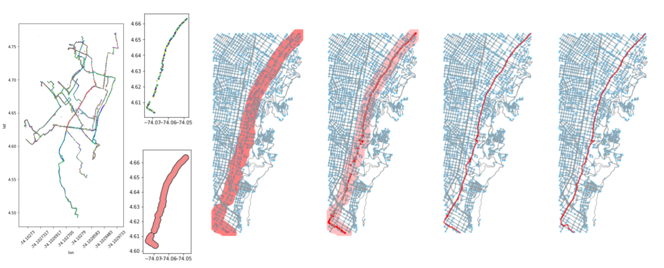
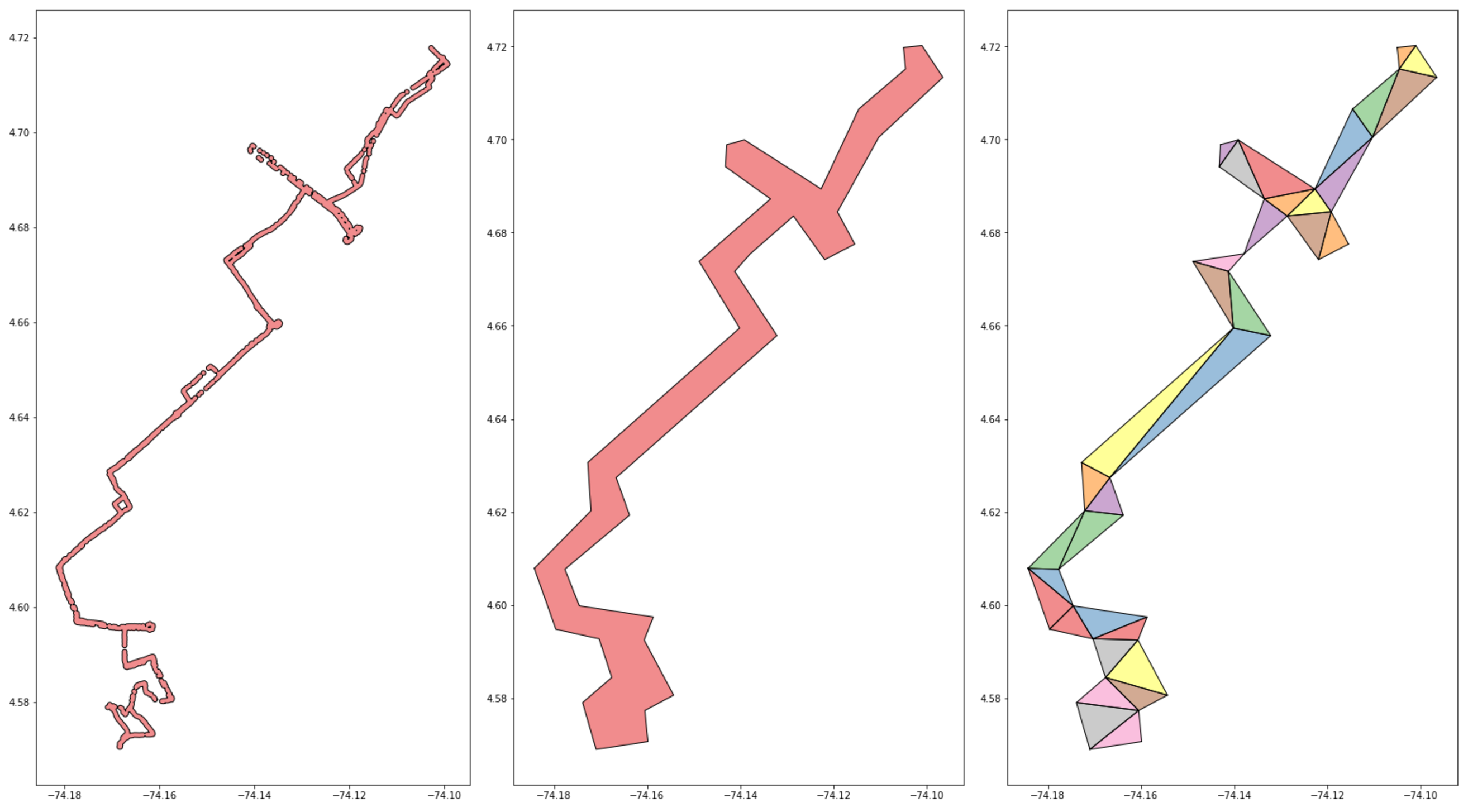
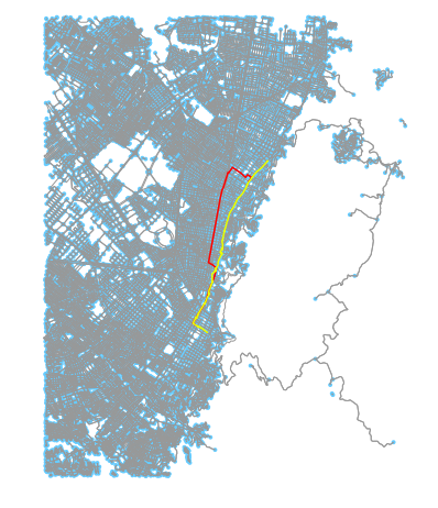
Above: A longest route being identified, extracted, and buffered. On the left, a subset of the total points array (to just one day) is shown.

Why do we want to pick the longest remaining trip ID from the remaining unused trip IDs? The reason we want to do so is that I’ve made the assumption that the longer the trip, the more likely it is to represent a hefty portion of a real route segment. As a result, it has the highest chance of catching all other trips along that unique route.

There is a serious weakness here, though. This whole method is premised on at least one trip having a complete path of the route mapped. This can be solved by improving the pairing mechanism in part 4.

Iteration part 3

Once we have the ID of the longest of the remaining trips, we use the extract_single_trip method to pull that trip out from the cleaned data frame and to convert its coordinates to points. From those points, we can construct a GeoSeries in Pandas and take that and buffer the resulting shapes to create a union single polygon of that route. 
There are two TODO items with this method. The first is that the buffer amount is hard set at the top of the ft_utils file. We should enable threading it through to the method as a parameter and thus allow the function to override the default. Secondly, the method should be improved to convert the points array first to a Shapely LineString object before the buffering operation is performed. We can safely sort the trip path because it is sorted by date time. Failure to do this occasionally can result in a MultiPolygon being created because the buffer distance is not sufficient to capture distance between two points in the route. This causes all sorts of downstream issues that could easily be handled by better geometry control at this step.

Iteration part 4

Now we start to enter the part of this workflow that becomes a bit laborious and slow in Python. Suffice to say, this is an area that is ripe for optimization in future refactoring.

In this portion of the iteration, we use get_similar_routes to pull out all unique trips that are deemed “related” to the reference trip. This method accomplishes this by first converting the cleaned reference data frame into a GeoDataFrame. As an aside, this is actually not that expensive of a step, but there is no reason to do it on every iteration; it could be stored and retrieved on each run.

With that new GeoDataFrame, we can group by trip ID and create new trip splines for each trip. Each trip is now stored as a LineString. Small, nonsense trips (e.g. a user accidentally started hitting record), are tossed. The threshold is set at 4 points (if something is less than 4 trips, ignore it). This could be increased, defensibly. I should also parameterize this sensitivity and allow it to be disabled altogether.

Each resulting LineString in the GeoDataFrame is then simplified. The simplification vector suppled to GEOS via Shapely’s API is hardcoded at 0.005. Again, this ought to be parametrized. The result is, like with the reference new unique trip we are comparing all these trips against, buffered (at 0.005, because we happen to be working in degrees projection, though I ought to have reprojected at meter-level).

Once we have the cleaned geometries for each of the data frame’s trips, we can get only those that intersect with the reference remaining longest trip:

df_int_gdf = df_gdf[df_gdf.intersects(reference_trip)]

This is another step that could be far improved. We should have more intelligent intersection. For example, if the reference trip is indeed the full length of the route, then we would need all other trips to match within a certain percent of overlap. Another idea would allow for a reference trip to not need to be the whole length of the trip would be to “grow” the reference shape by incrementally adding any trip IDs that overlap within a certain percentage threshold and then update the reference shape to that one.

Iteration part 5 - 8

With the resulting subset, we take the unique trip IDs and add them to the reference dictionaries that are keeping track of already assigned Trip IDs, as well as the object that keeps pairs together. The key for this dictionary will use the longest trip ID from Part 2 as it’s identifier. The route will end up using that trip ID as the basis for its unique ID downstream.

The print statements included in the utilities as well as the workflow outlined in the snippet above will result in a number of logs such as the below being printed. These can help you track progress as the loop runs through completion.

Starting new pass through. Elapsed time: 15 min
Good vals remaining: 236
Using this target trip: T88248718
Subset that intersect target trip:  288
Of that subset, 25 are valid
Identified 25 trip IDs: ['T24651929', ... ‘T19859556']

Routes generation performance

For the Bogota dataset, the run time was about 35 minutes. This could be improved by a number of currently pending optimizations. It also go up if the less naive intersection identification subsetting process from Part 4 that I outlined were implemented.

There are opportunities to parallelize this process for speed gains. If you look back at some of my previous posts, I’ve done work in parallelizing GeoPandas operations via Dask’s Distributed library. This, with a few EC2 instances can convert a 30 minute process into one that takes seconds. It’s critical, though, to use the Distributed utility as simply running a multithreaded Python operation can actually result in lower performance than just a single threaded operation. If you are curious about this, feel free to Google about Python’s GIL (global interpreter lock) and its limitations, but its discussion is out of scope for this post.

Discrete route extraction

The unique_trip_id_pairs dictionary now has a set of keys which are the reference trip IDs and within them all the paired points. From these groupings, we can generate point clouds:

sub_df = bdfc[bdfc['trip_id'].isin(tids)]
sub_xys = [Point(x, y) for x, y in zip(sub_df['lon'].values, sub_df['lat'].values)]
sub_gdf = gpd.GeoDataFrame(sub_df, geometry=sub_xys)

Each point cloud consists of all routes that are within that trip’s pairings. Note that here is another unnecessary recreation of the reference layer GeoDataFrame. That said, this is hardly the main performance bottleneck, as you will see in a moment.

Simplifciation

Once we have that subset, we run the following utility method to generate a simplified shape of the points that are in the subsetted data frame:

simplified = ft.unify_trips(sub_gdf.geometry, 0.0025)

unify_trips takes that list of points and buffers them by the second parameter variable. It then converts that into a MultiPolygon and takes the largest of the Polygons. This helps handle situations where there are hanging points that lie outside the main “blob.”

Here is an example of that happening:

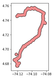
In that example case, we would end up with two Polygons. We take the larger and simply toss the smaller. Once we have that larger, we return it, simplified (largest.simplify(0.0001)). Again, this is a parameter that needs to be parameterized. You can also see that I’ve been working in degrees projection (generally ill-advised, but this is just a sketch of the process as a working concept).

Triangulation

Now we get to run a triangulation process to convert the geometry into a series of triangle elements. This is another area that needs a great deal more refinement. There is a Python library Tri that allows for constrained Delaunay Triangulation, but it’s quite brittle. I outlined how it works in a previous post if you are interested in knowing more.

# Convert this polygon into a triangulated composition
tri_cleaned = ft.triangulate_path_shape(simplified)

This method skips the use of the constrained method and just uses GEOS’s built in triangulation method which is bound via Shapely’s triangulate API function. The result typically works to return a shape where triangles are drawn between all points along the edge of the shape.

This result is not 100% guaranteed, though. I discovered that and made a note of it on the Shapely repo here. Through that discussion we found that this observed and reported behavior was reasonable. It is for this reason that a stable implementation of a constrained triangulation method in Python would be quite valuable. This would be a time intensive project, but one I might be interesting in diving into more, having been exposed to this issue. Again, if you refer to that issues conversation, you will see that an equivalent method has been built out in Java. Potentially integrating a Java component to this workflow to execute that portion of the analysis may be the most viable path forward in the short term.

We can see hints at this issue from the above image. The above triangulation method is not rock solid. We an see instances where triangles that ought to be returned are not. There is a chance that a disconnected MultiPolygon could be returned.

Above, the issue in greater detail, circled in red.

So why are we performing this triangulation? Again, for more detail it is best to see previous posts on this topic, but you can generate shortest paths from these triangulations that will provide us with a discreet spline for this group of routes.

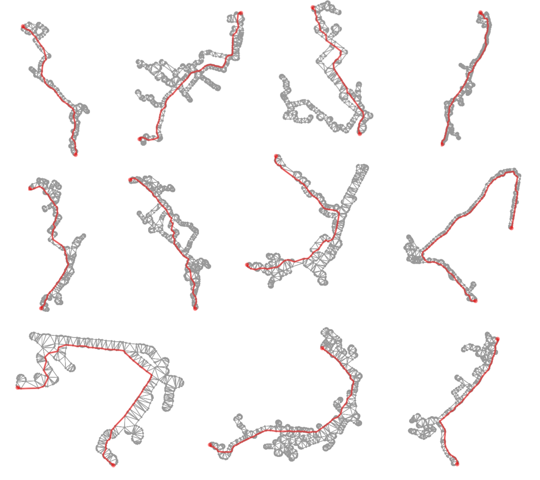
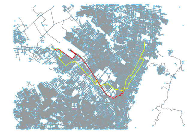
Above: Examples of shortest paths being calculated using the triangulation output as a graph network to identify potential route splines.

Although these paths may be slightly off from where the “real” road network would be, they are within a defensible margin of area. Most importantly, for performing service analyses of networks and transit systems, they are within a roughly 5-minute minute walk radius from the actual spline at any point at this buffer level. This is sufficient for calculating coverage, service levels, and accessibility within a region, defensibly. If a truly accurate route path shape is desired, then we must dive into a creating a converter that takes these shapes and best snaps them to the OSM network (as well as deals with inaccuracies in the OSM network). This is out of scope for the intent of this post and the problem trying to be solved.

It definitely is something worth looking into later, though.

Skeletonization

Once we have the triangulated the geometry, we are still missing 2 values before we can actually generate those shortest paths for each triangulated route shape shown above. What we still need is a “start” and an “end” point. There’s a couple of ways to the get the two farthest points on a geometry and what I ended up landing on was Polyskel: Polyskel is a Python 2 implementation of the straight skeleton algorithm as described by Felkel and Obdržálek in their 1998 conference paper “Straight Skeleton Implementation.” You can learn more about it by visiting the Github repository.

It is included in its entirety in the ft_bogota repo. Slight modifications have been made to it (and the Pyeuclid library that it relies on) to allow them to run in Python 3. The method takes a geometry and identifies the least number of lines that extends to each of the polygon’s vertices and then the least number of lines that connects those points to an internal, “central” spline.

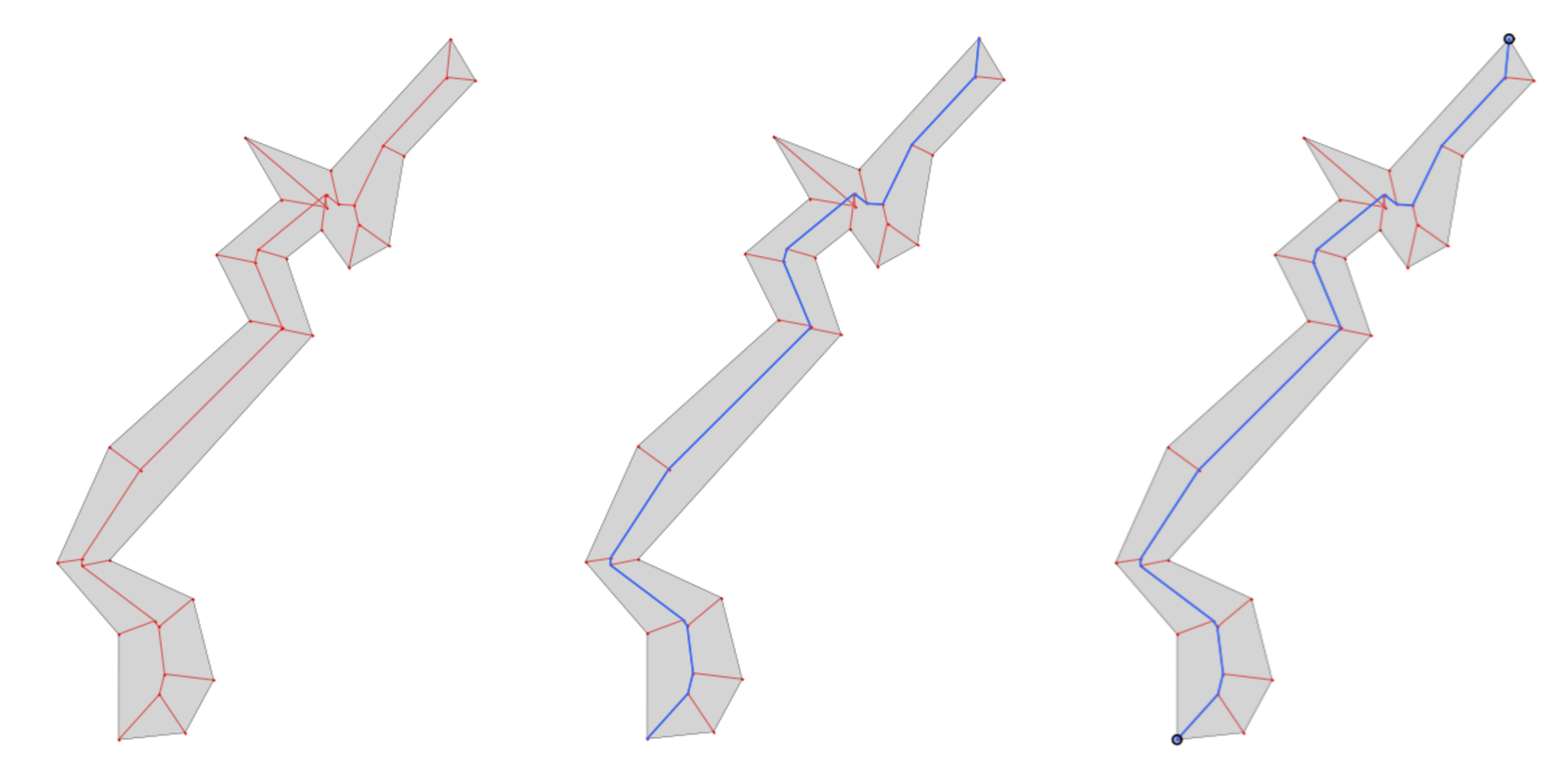
In the interest of somewhat containing the length of this post, I won’t dive too much in to how this work and can save that for a later post. Suffice to say, if you look at the example in the above image, I can then take these limited edges and convert them to a NetworkX graph. With that NetowrkX graph, I can identify all possible paths in that network and select the longest one. This is the path whose extremities are essentially the “start” and “end” points of the parent geometry.

Identifying route splines

Once we have the skeletonization results (two farthest points within a geometry), running the longest route method is easy:

first_point, last_point = ft.get_farthest_point_pair(skeleton)

The above method simply converts the triangulated geometry into a NetworkX graph and uses the triangle edges as graph edges. NetworkX is a pure Python implementation of a network graph analyses tool that was started (and I believe continues to be supported by) Los Alamos Labs since the early 2000s. An improvement here would be to not introduce redundancies between triangle edges so that graphs can be constructed and navigated more quickly. This will help speed up this step.

Route imputation performance

This process is slow; really slow. On the 24 routes from the Bogota dataset, execution time was about 3 minutes each (so a little over an hour for the whole set). A great deal of work could be done to optimize these steps. I’ll note the low hanging fruit in each section as I describe the overall structure throughout the remainder of this post.

---
Working with reference trip id T64293761 (15/24).
Already calculated. Skipping...
Elapsed time: 22 min
Unified polygons: 2. Largest will be extracted.

If you use the notebook’s method and the library’s logs, you will see status updates for each that look similar to the above.

Using the results

The result of the operation will result in all routes separated. Loading them into GeoPandas will enable you to work with each as you would another other Shapely object. The above plot was generated by simply converting the routes into a GeoDataFrame and plotting over a shape of the administrative boundaries of Bogota, Colombia.

Simply buffering that geometry was what enabled me to perform simple analyses like seeing how much of the area of the city was services by these routes:

route_service_area = []
for r_key in list(results.keys()):
    path = results[r_key]['path']
    path_coverage_zone = path.buffer(0.0035)
    
    route_service_area.append(path_coverage_zone) 

coverage_area = (gpd.GeoSeries(route_service_area)
                 .unary_union
                 .intersection(bogota_shape).area)
coverage_area/bogota_shape.area
# 0.6348142862773293

Example spatial analysis with the resulting data

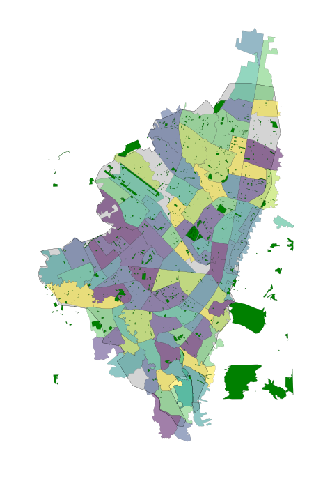
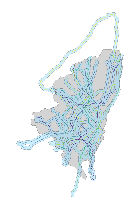
We can use the UPZs from earlier and load them in, as well as parks and open space data gleaned from OpenStreetMap to create a base canvas on which to determine what portion of the population these routes serve. The UPZ shapes have population data associated with them.

All we need to do is take the routes and buffer them by a ten minute walk time. Once we do that, we can remove the areas that are park space (where we can presume people do not live), and then generate a new geometry of the difference. The components of this are shown in the above image.

Intersecting this with the UPZs, we can then pull out the portion of each area of the UPZs that are covered in that walk radius. Using that as an area proportion, we can glean minimum and maximum coverage of UPZs (as much as 99.8% and as little as 0%), or what portion of the population, roughly, is serviced by these routes (59.7%).

What’s next?

The shapes are only rough. It would be nice to have routes that line up with the OSM network data. In order to do this there may need to be a “by-hand” portion. I can load these geometries up into a map and use Mapzen or Mapbox’s map matching API to tweak the routes until they satisfy a visual inspection. I can easily set up a local QA tool to do this that works through each route and loads in the geometry as a GeoJSON and attempts a naive map match that I can then tweak by dragging the points around a map until it looks satisfactory.

Other than that, it is important to note that this is just a sketch of a framework. I have identified a number of points here that are brittle. Each of these could easily thrown a wrench in the workflow for any number of edge cases and working through how these are handled will be a great deal of work. Some already have been handled, though, and this system does successfully run from end to end with the Bogota dataset.

More on map matching

For a variety of reasons, map matching is not wholly reliable at present. For one, the data we are putting in is quite noisy and the splines generated are averages of that. Because of that, they are inherently inaccurate. On a busy street network like the one in Bogota, it’s easy for the route to be misplaced on a neighboring street.

Above: 2 examples of map matched paths using Mapzen’s API. Currently there are some limitations to the algorithm (and to the data being supplied).

Also interesting is the tendency for routes to occasionally fall quite off course. There are a couple of issues causing this. Some roads listed as one-way in OSM appear to be two way. In addition, our shape generator does not account for direction and might place a path in an incorrect location if the route tends to use one road in one direction and another when in reverse.

One of the core checks of the Mapzen matching API is to penalize potential routes that are far off course and whose distance thus exceeds the distance of the input path. What’s interesting is that on nuanced networks a route that is similarly distanced but clearly off route can potentially “slip through” the cracks, as we see in the above two examples.

GTFS

In the next post, I will outline how we can then take that original trace data and derive time cost between each route segment.

Continue to the second section

This concludes the first part in a two-part series. The second section is located here: Tethering Schedules to Routes via Trace Data.

This is part of a 4 part series, realted to deep diving into Flocktracker Bogota data. All 4 parts in the series are:

• Cleaning and Analysis of Bogota Flocktracker Data
• Programmatic Geometry Manipulation to Auto-generate Route Splines
• Tethering Schedules to Routes via Trace Data
• Synthesizing Multiple Route Trace Point Clouds